Title 40 CFR Part
191
Subparts B and C
Compliance Recertification
Application
for the
Waste Isolation Pilot Plant
Appendix TFIELD-2009
Transmissivity Fields
United States Department
of Energy
Waste Isolation Pilot Plant
Carlsbad Field Office
Carlsbad, New Mexico
Appendix TFIELD-2009
Transmissivity Fields
TFIELD-1.0 Overview of Transmissivity Field Development, Calibration, and Modification Process
TFIELD-2.0 Development of Maps of Geologic Factors
TFIELD-3.0 Development of Model Relating Culebra Transmissivity to Geologic Factors
TFIELD-3.1 Fracture Interconnection
TFIELD-3.2 Overburden Thickness
TFIELD-3.4 Halite Overlying the Culebra
TFIELD-3.5 Halite Bounding the Culebra
TFIELD-3.6 High-Transmissivity Zones
TFIELD-3.7 Linear Transmissivity Model
TFIELD-3.8 Linear-Regression Analysis
TFIELD-4.0 Calculation of Base T Fields
TFIELD-4.1 Definition of Model Domain
TFIELD-4.2 Reduction of Geologic Map Data
TFIELD-4.3 Indicator Variography
TFIELD-4.4 Conditional Indicator Simulation
TFIELD-4.5 Construction of Base Transmissivity Fields
TFIELD-5.0 Construction of Seed Realizations
TFIELD-6.0 T-Field Calibration to Steady-State and Transient Heads
TFIELD-6.1 Modeling Assumptions
TFIELD-6.3 Boundary Conditions
TFIELD-6.4 Observed Steady-State and Transient Head Data Used in Model Calibration
TFIELD-6.5 Spatial Discretization
TFIELD-6.6 Temporal Discretization
TFIELD-6.7 Weighting of Observation Data
TFIELD-6.8 Assignment of Pilot Point Geometry
TFIELD-6.9 Stochastic Inverse Calibration
TFIELD-7.0 T-Field Acceptance Criteria
TFIELD-7.1 Candidate Acceptance Criteria
TFIELD-7.1.2 Fit to Steady-State Heads
TFIELD-7.1.4 Fit to Transient Heads
TFIELD-7.2 Application of Criteria to T Fields
TFIELD-7.2.2 Fit to Steady-State Heads
TFIELD-7.2.4 Fit to Transient Heads
TFIELD-7.3 Final Acceptance Criteria
TFIELD-8.0 Inverse Modeling Results
TFIELD-8.2 Fit to Steady-State Heads
TFIELD-8.3 Pilot-Point Sensitivity
TFIELD-8.4 Ensemble Average T Field
TFIELD-9.0 Modification of T Fields For Mining Scenarios
TFIELD-9.1 Determination of Potential Mining Areas
TFIELD-9.2 Scaling of Transmissivity
Figure TFIELD-1. Structure Contour Map for the Top of the Culebra
Figure TFIELD-2. Salado Dissolution Margin
Figure TFIELD-3. Rustler Halite Margins. See Figure TFIELD-4 for Key to Stratigraphic Column.
Figure TFIELD-4. Stratigraphic Subdivisions of the Rustler
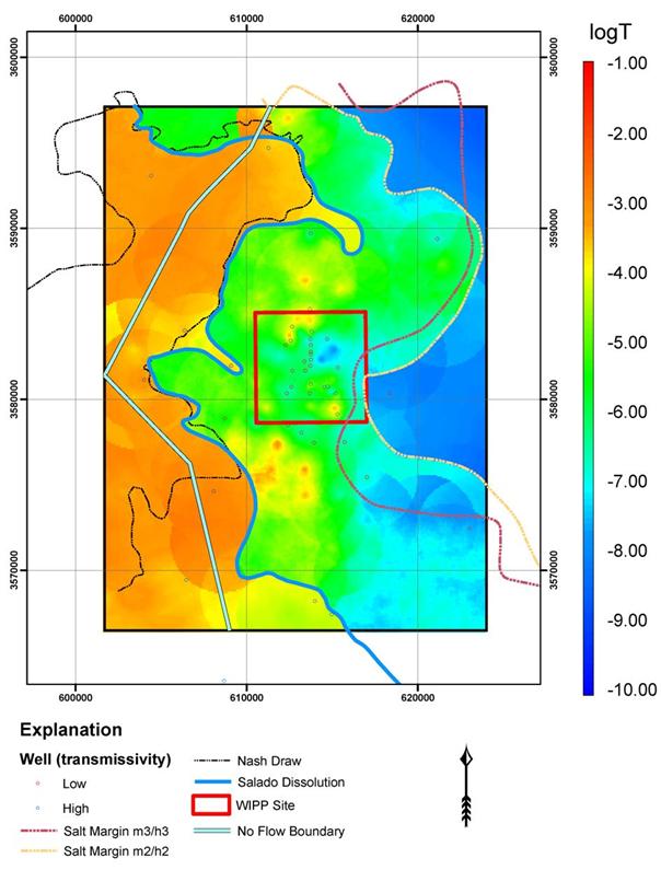
Figure TFIELD-6. Well Locations and log10 Culebra Transmissivities
Figure TFIELD-7. Regression Fit to Observed Culebra log10 T Data
Figure TFIELD-8. Zones for Indicator Grids
Figure TFIELD-9. High-T Indicator Model and Experimental Variograms
Figure TFIELD-10. Soft Data Around Wells
Figure TFIELD-11. Example Base T Field
Figure TFIELD-17. Gaussian Trend Surface Fit to the 2000 Observed Heads
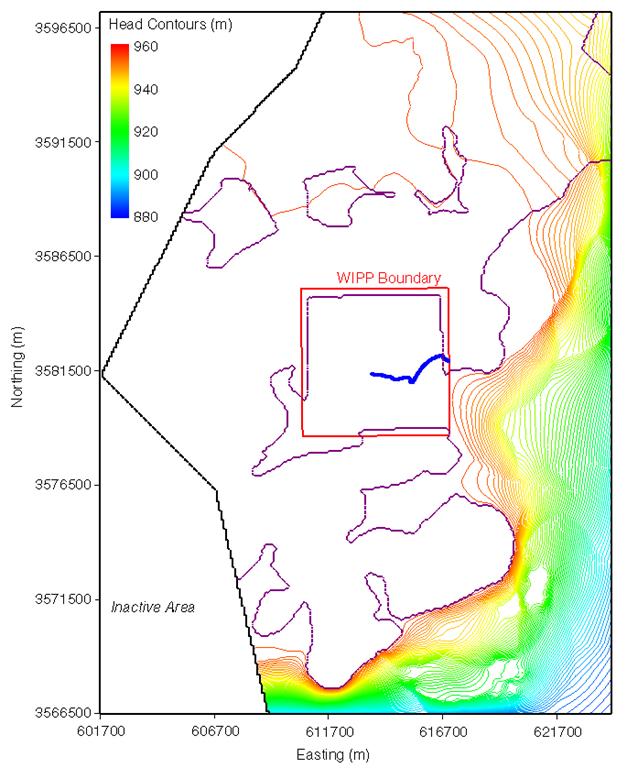
Figure TFIELD-21. Values of Fixed Heads Along the Eastern Boundary of the Model Domain
Figure TFIELD-23. Locations of the H-3b2 Hydraulic Test Well and Observation Wells
Figure TFIELD-24. Observed Drawdowns for the H-3b2 Hydraulic Test
Figure TFIELD-25. Locations of the WIPP-13 Hydraulic Test Well and Observation Wells
Figure TFIELD-27. Locations of the P-14 Hydraulic Test Well and Observation Wells
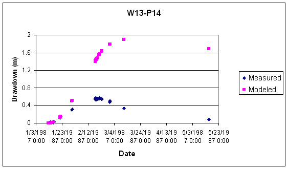
Figure TFIELD-28. Observed Drawdowns for the P-14 Hydraulic Test
Figure TFIELD-29. Locations of the WQSP-1 Hydraulic Test Well and Observation Wells
Figure TFIELD-30. Observed Drawdowns for the WQSP-1 Hydraulic Test
Figure TFIELD-31. Locations of the WQSP-2 Hydraulic Test Well and Observation Wells
Figure TFIELD-32. Observed Drawdowns from the WQSP-2 Hydraulic Test
Figure TFIELD-33. Locations of the H-11 Hydraulic Test Well and Observation Wells
Figure TFIELD-34. Observed Drawdowns for the H-11 Hydraulic Test
Figure TFIELD-35. Locations of the H-19 Hydraulic Test Well and Observation Wells
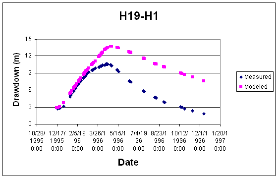
Figure TFIELD-36. Observed Drawdowns From the H-19 Hydraulic Test
Figure TFIELD-38. Locations of the Adjustable and Fixed Pilot Points Within the Model Domain
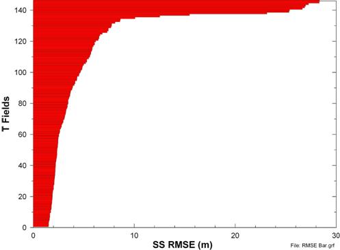
Figure TFIELD-44. Steady-State RMSE Values for 146 T Fields
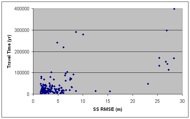
Figure TFIELD-45. Steady-State RMSE Values and Associated Travel Times
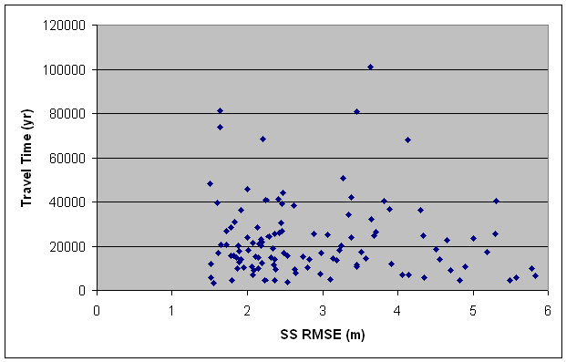
Figure TFIELD-46. Travel Times for Fields with Steady-State RMSE <6 m (20 ft)
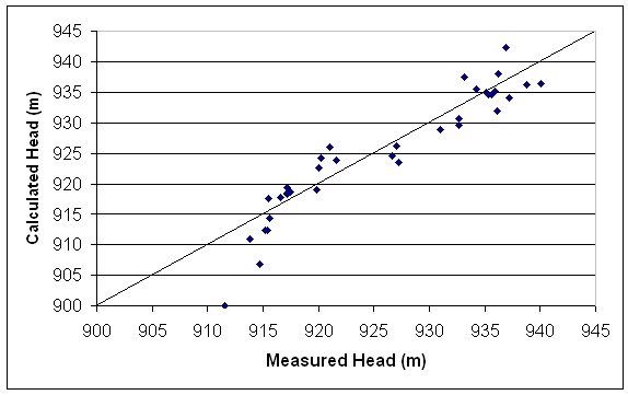
Figure TFIELD-47. Measured Versus Modeled Steady-State Heads for T Field d21r10
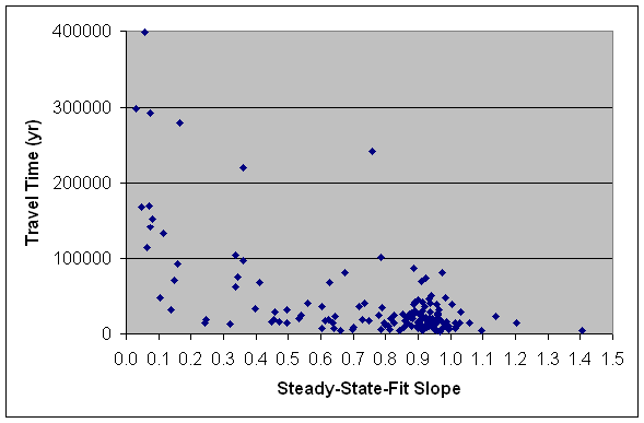
Figure TFIELD-48. Steady-State-Fit Slope Versus Travel Time for All Fields
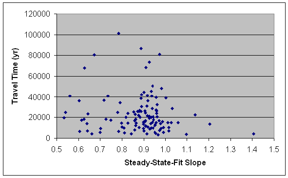
Figure TFIELD-49. Steady-State-Fit Slope Versus Travel Time for Slopes >0.5
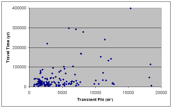
Figure TFIELD-50. Transient Phi Versus Travel Time for All Fields
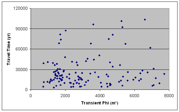
Figure TFIELD-51. Transient Phi Versus Travel Time for Phi <8,000 m2
Figure TFIELD-52. Example of Passing Well Response from T Field d21r10
Figure TFIELD-53. Example of Failing Well Response from T Field d21r10
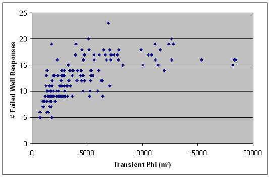
Figure TFIELD-54. Transient Phi Versus Number of Failed Well Responses
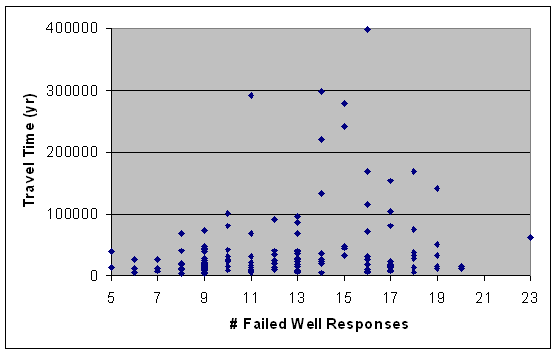
Figure TFIELD-55. Number of Failed Well Responses Versus Travel Time
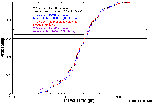
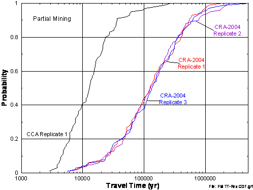
Figure TFIELD-56. Travel-Time CDFs for Different Sets of T Fields
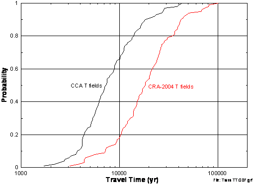
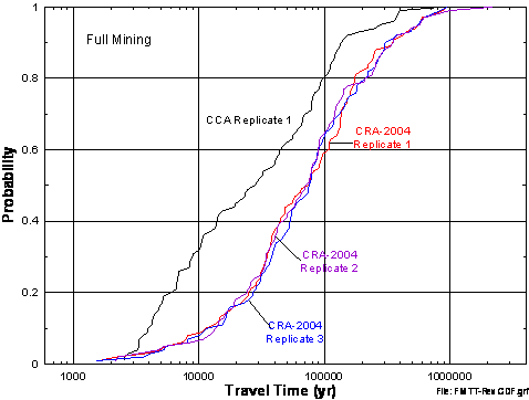
Figure TFIELD-57. Travel-Time CDFs for CCA and CRA-2004 T Fields
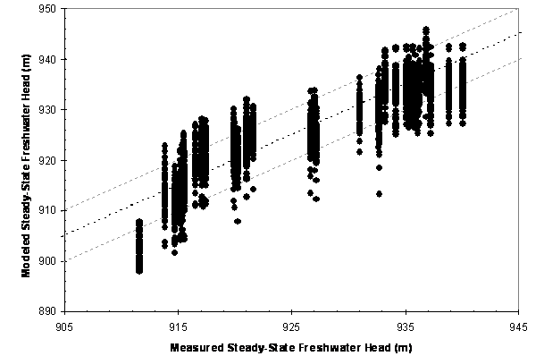
Figure TFIELD-60. Scatterplot of Measured Versus Modeled Steady-State Heads
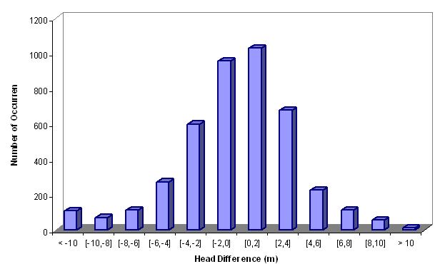
Figure TFIELD-61. Histogram of Differences Between Measured and Modeled Steady-State Heads
Figure TFIELD-64. Ensemble Average of 121 Calibrated T Fields
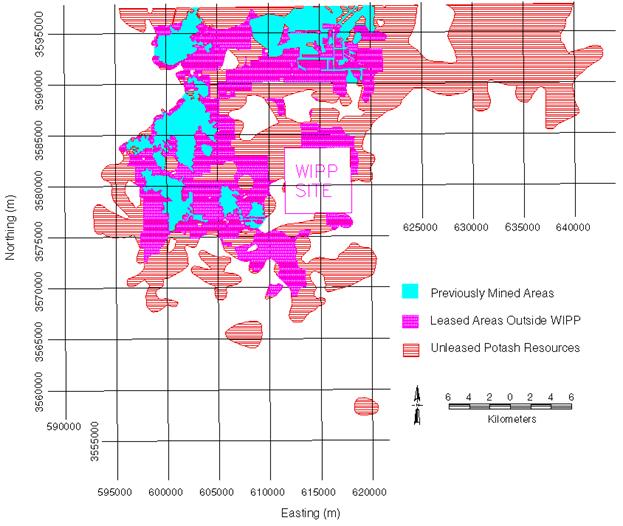
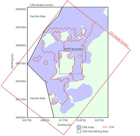
Figure TFIELD-66. Potash Resources Near the WIPP Site
Figure TFIELD-68. Comparison of CRA-2004 and CCA Areas Affected by Mining
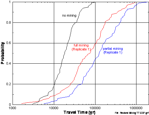
Figure TFIELD-69. CDFs of Travel Times for the Full-, Partial-, and No-Mining Scenarios
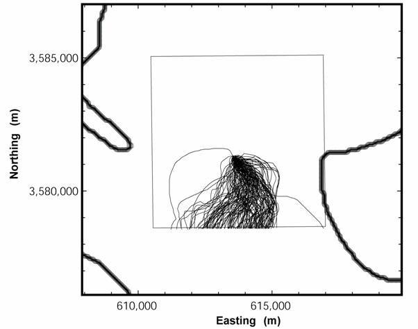
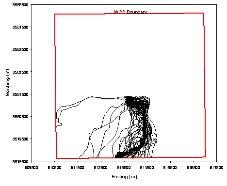
Figure TFIELD-73. Particle Tracks for Replicate 1 for the Partial-Mining Scenario
Figure TFIELD-74. Particle Tracks for Replicate 2 for the Partial-Mining Scenario
Figure TFIELD-75. Particle Tracks for Replicate 3 for the Partial-Mining Scenario
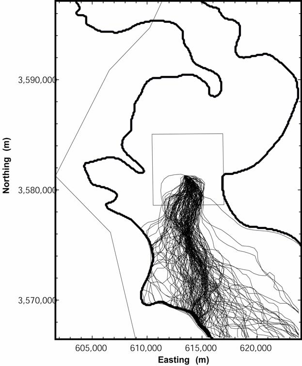
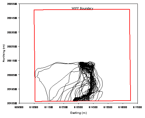
Figure TFIELD-76. Particle Tracks for Replicate 1 for the Full-Mining Scenario
Figure TFIELD-77. Particle Tracks for Replicate 2 for the Full-Mining Scenario
Figure TFIELD-78. Particle Tracks for Replicate 3 for the Full-Mining Scenario
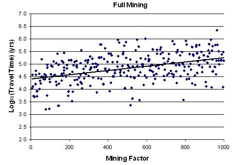
Figure TFIELD-79. Correlation Between the Random Mining Factor and log10 of Travel Time
Table TFIELD-1. Regression Coefficients for Equations (TFIELD.2) and (TFIELD.3)
Table TFIELD-2. Coordinates of the Numerical Model Domain Corners
Table TFIELD-6. Parameters for the Gaussian Trend Surface Model Fit to the 2000 Heads
Table TFIELD-7. Model Variogram Parameters for the Head Residuals
Table TFIELD-8. Transient Hydraulic Test and Observation Wells for the Drawdown Data
Table TFIELD-10. Observation Weights for Each of the Observation Wells
Table TFIELD-11. Summary Information on T Fields
Table TFIELD-12. T-Field Transmissivity Multipliers for Mining Scenarios
Appendix TFIELD-2009 and the associated transmissivity fields for Compliance Recertification Application (CRA)-2009 were originally prepared for the CRA-2004 Performance Assessment Baseline Calculation. The only changes that have been made to the text are minor and editorial in nature, such as corrections of referencing errors and the addition of a missing reference. Although additional hydrogeologic investigations, described in Appendix HYDRO-2009, were performed after these transmissivity fields (T fields) were constructed, T fields incorporating the new data have not been completed.
% percent
AP Analysis Plan
BLM Bureau of Land Management
CCA Compliance Certification Application
CDF cumulative distribution function
CRA Compliance Recertification Application
DOE U.S. Department of Energy
EPA U.S. Environmental Protection Agency
ft feet
ft2 square feet
GHz gigahertz
GSLIB Geostatistical Software Library
high-T high-transmissivity
km kilometer
LHS Latin hypercube sampling
low-T low-transmissivity
LWB Land Withdrawal Boundary
m meter
m2 square meters
M/H mudstone/halite
m2/s square meters per second
m3/s cubic meters per second
mi mile
PA performance assessment
PEST Parameter ESTimation software
RMSE root mean squared error
s second
S storativity
SNL Sandia National Laboratories
SP stress period
SSE sum of squared errors
T field transmissivity field
USGS United States Geological Survey
UTM Universal Transverse Mercator
WIPP Waste Isolation Pilot Plant
WQSP Water Quality Sampling Program
Modeling the transport of radionuclides through the Culebra Dolomite Member of the Rustler Formation (hereafter referred to as the Culebra) is one component of the Performance Assessment (PA) performed for the Waste Isolation Pilot Plant (WIPP) Compliance Recertification Application (CRA). This transport modeling requires a model of groundwater flow through the Culebra. This Appendix describes the process used to develop and calibrate the transmissivity fields (T fields) for the Culebra, and then modify them for the possible effects of potash mining for use in flow modeling for the CRA-2004 (U.S. Department of Energy 2004).
The work described in this appendix was performed under two Sandia National Laboratories (SNL) Analysis Plans (APs): AP-088 (Beauheim 2002a) and AP-100 (Leigh, Beauheim, and Kanney 2003). AP-088 (Analysis Plan for the Evaluation of the Effects of Head Changes on Calibration of Culebra T Fields) dealt with the development, calibration, and modification for potash mining of the T fields. AP-100 (Analysis Plan for Calculations of Culebra Flow and Transport: Compliance Recertification Application) included the development of T-field acceptance criteria, as well as radionuclide-transport calculations not described herein.
The starting point in the T-field development process was to assemble information on geologic factors that might affect Culebra transmissivity (Section TFIELD-2.0). These factors include dissolution of the upper Salado Formation, the thickness of overburden above the Culebra, and the spatial distribution of halite in the Rustler Formation above and below the Culebra. Geologic information is available from hundreds of oil and gas wells and potash exploration holes in the vicinity of the WIPP site, while transmissivity values are available from only 46 well locations. Details of the geologic data compilation are given in Powers (2002a, 2002b, 2003) and summarized below in Section TFIELD-2.0.
A two-part “geologically based” approach was then used to generate Culebra base T fields. In the first part (Section TFIELD-3.0), a conceptual model for geologic controls on Culebra transmissivity was formalized, and the hypothesized geologic controls were regressed against Culebra transmissivity data to determine linear regression coefficients. The regression includes one continuously varying function, Culebra overburden thickness, and three indicator functions that assume values of 0 or 1 depending on the occurrence of open, interconnected fractures, Salado dissolution, and the presence or absence of halite in units bounding the Culebra.
In the second part (Section TFIELD-4.0), a method was developed for applying the linear regression model to predict Culebra transmissivity across the WIPP area. The regression model was combined with the maps of geologic factors to create 500 stochastically varying Culebra base T fields. Details about the development of the regression model and the creation of the base T fields are given in Holt and Yarbrough (2002, 2003a, 2003b).
By the nature of regression models, the base T fields do not honor the measured transmissivity values at the measurement locations. Therefore, before these base T fields could be used in a flow model, they had to be conditioned to the measured transmissivity values. This conditioning is described in McKenna and Hart (2003a, 2003b) and summarized in Section TFIELD-5.0. Section TFIELD-6.0 presents details on the modeling approach used to calibrate the T fields to both steady-state heads and transient drawdown measurements. Heads measured in late 2000 were used to represent steady-state conditions in the Culebra, and drawdown responses in 40 wells to pumping in 7 wells were used to provide transient calibration data. Details on the heads and drawdown data used are described in Beauheim (2002b) and Beauheim and Fox (2003). Assumptions made in modeling, the definition of an initial head distribution, assignment of boundary conditions, discretization of the spatial and temporal domain, weighting of the observations, and the use of Parameter ESTimation software (PEST) (Doherty 2002) in combination with MODFLOW-2000 (Harbaugh et al. 2000) to calibrate the T fields using a pilot-point method are described in McKenna and Hart (2003a, 2003b) and summarized in Section TFIELD-6.0.
Section TFIELD-7.0 addresses the development and application of acceptance criteria for the T fields. Acceptance was based on a combination of objective fit to the calibration data and providing travel time results consistent with the cumulative distribution function (CDF) of travel times from the 23 best-calibrated T fields (Beauheim 2003). Of the 146 T fields that went through the calibration process, 121 T fields were judged adequate for further use, with the 100 best T fields selected for use in the CRA-2004 transport calculations.
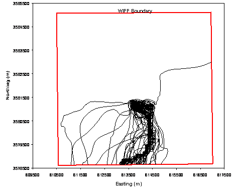
Section TFIELD-8.0 provides summary statistics and other information for the 121 T fields that were judged to be acceptably calibrated. Particle tracks from a point above the center of the WIPP disposal panels to the Land Withdrawal Boundary (LWB) are shown, along with information on the model fits to steady-state heads, identification of the most sensitive pilot point locations, and characteristics of an ensemble average T field. This information is summarized from McKenna and Hart (2003b).
Section TFIELD-9.0 discusses the modification of the T fields to account for the effects of potash mining both within and outside the WIPP LWB. Mining-affected areas were delineated, random transmissivity multipliers were applied to transmissivities in those areas, and particle tracks and travel times were determined (Lowry 2003). The flow fields produced by these mining-affected T fields are input to SECOTP2D for the CRA-2004 radionuclide-transport calculations.
Section TFIELD-10.0 provides a brief summary of this appendix.
Beauheim and Holt (1990), among others, suggested three geologic factors that might be related to the transmissivity of the Culebra in the vicinity of the WIPP site:
1. Thickness (or erosion) of overburden above the Culebra
2. Dissolution of the upper Salado
3. Spatial distribution of halite in the Rustler below and above the Culebra
Culebra transmissivity is inversely related to thickness of overburden because stress relief associated with erosion of overburden leads to fracturing and opening of preexisting fractures. Culebra transmissivity is high where dissolution of the upper Salado has occurred and the Culebra has subsided and fractured. Culebra transmissivity is observed to be low where halite is present in overlying and/or underlying mudstones. Presumably, high Culebra transmissivity leads to dissolution of nearby halite (if any). Hence, the presence of halite in mudstones above and/or below the Culebra can be taken as an indicator for low Culebra transmissivity.
Maps were developed for each of these factors using drillhole data of different types. The general area for the geologic study comprised 12 townships, located in townships T21S to T24S, ranges R30 to 32E (the WIPP site lies in T22S, R31E). The original sources of geologic data for this analysis are mainly Powers and Holt (1995) and Holt and Powers (1988) and new information derived by log interpretation by Powers (2002a, 2002b, 2003). All of the data are either included or summarized in the references cited above, and can be independently checked; basic data reports are available for WIPP drillholes, geophysical logs for oil and gas wells are available commercially or at offices of the Oil Conservation Division (New Mexico) in Artesia and Hobbs, and potash drillhole information is in files that can be accessed for stratigraphic information at the Bureau of Land Management (BLM), Carlsbad, NM. No proprietary data are included.
Factor 1 is represented by a structure contour map of the elevation of the top of the Culebra (Figure TFIELD-1) that can be digitized and then subtracted from a digital elevation model of the land surface to obtain the thickness of overburden. Factor 2 is represented on a map as an approximate margin of the area beginning to be affected by dissolution of the upper Salado (Figure TFIELD-2). Factor 3 is delineated on a map by lines that represent as nearly as possible the boundaries of the occurrence of halite in the Los Medaños, Tamarisk, and Forty-niner Members of the Rustler in the study domain (Figure TFIELD-3).
With respect to Factor 2, the upper Salado has been dissolved, and presumably is still dissolving, along the eastern margin of Nash Draw. On the basis of limited core information, Holt and Powers (1988) suggested that formations overlying the dissolving upper Salado in Nash Draw are affected in proportion to the amount of Salado dissolution. The most direct way to estimate the spatial distribution of dissolution is to have cores of the upper Salado and basal Rustler and knowledge of the thickness to marker beds in the upper Salado. The upper Salado has not been cored frequently, but geophysical logs from oil and gas wells, and descriptive logs of cores or cuttings from potash drillholes, provide a considerable amount of evidence of the thickness of the lower Rustler and upper Salado, even though cores and cuttings are no longer available from potash industry drillholes.
Figure TFIELD-1. Structure Contour Map for the Top of the Culebra
Figure TFIELD-2. Salado Dissolution Margin
Figure TFIELD-3. Rustler Halite Margins. See Figure TFIELD-4 for Key to Stratigraphic Column.
Potash industry geological logs examined at the BLM in Carlsbad, NM, are quite variable in the quality of description and the stratigraphic interval described. Drillhole logs from the 1930s and 1950s typically are the most descriptive; recent drillhole logs are commonly useless for this project because no strata are described above portions of the McNutt potash zone of the Salado, near the middle of the formation.
The top of the Culebra and the base of the Vaca Triste Sandstone Member in the upper Salado are the most consistent stratigraphic markers spanning the upper Salado that are recognizable across various types of records. As a guide to the limits or bounds of upper Salado dissolution, a map of the thickness from the top of Culebra to the base of Vaca Triste was prepared (Powers 2003). In conjunction with previous work by Powers and Holt (1995) and the evidence of the structure of the top of Culebra (see Figure TFIELD-1), an approximate boundary of dissolution was drawn as shown in Figure TFIELD-2.
With respect to Factor 3, the boundaries of where halite is found in the three non-carbonate members of the Rustler have been drawn several times on the basis of different borehole data sets and different data types (e.g., core data and geophysical logs). For the most part, the different versions of the boundaries do not vary significantly. In the map shown in Figure TFIELD-3, the margins are based principally on the work of Powers and Holt (1995), which is a continuation of work reported by Holt and Powers (1988). As discussed in Powers and Holt (1995), the boundaries drawn here vary slightly from those drawn by Snyder (1985) based on core data for two reasons: (1) the Los Medaños Member (Powers and Holt 1999; formerly called the unnamed lower member) is here divided into two separate halite-bearing units (Powers and Holt 2000), and (2) geophysical log signatures are now used to identify halite in areas where cores are not available. Figure TFIELD-3 includes a stratigraphic sketch showing the relationship of halite-bearing strata to other strata in the Rustler. Following the convention established by Holt and Powers (1988), the mudstone/halite (M/H) strata are numbered consecutively starting at the base of the Rustler.
The margins for halite have now been drawn in the area north of the WIPP site around the northeastern arm of Nash Draw based on the descriptions of halite encounters in the Rustler Formation in potash drillholes. In addition, a few areas have been modified (from Powers and Holt 1995) to the south and west of the WIPP based on the records from potash drillholes as well as the records of drilling H-12 and H-17 for the WIPP.
In 12 potash drillholes, halite was reported above the upper contacts of the Culebra or Magenta Dolomite Members. The boundaries for M3/H3 and M4/H4 margins (i.e., the spatial limits of where halite is found in the mudstone intervals) have been drawn north of the WIPP based on these data. The depth below the Culebra at which halite was reported has also been used to draw the boundaries of the lower (M1/H1) or the upper (M2/H2) halite-bearing units of the Los Medaños in this area. Anhydrite A1 divides the M1/H1 (below) and M2/H2 (above) intervals. M2 (no halite) is about 3 meters (m) (10 feet [ft]) thick. If halite is reported within about 3 m (10 ft) of the base of Culebra or is clearly above A1, H2 is considered to be present. The M1/H1 interval is about 33–37 m (110–120 ft) thick at the WIPP site. In potash drillholes north of the WIPP site, where halite was reported less than 33 m (110 ft) below the Culebra, H1 is present. Within the zone for H1, other drillholes frequently reveal halite less than 33 m (110 ft) below the Culebra.
It should be noted that the report of “top of salt” or first salt in records for potash drillholes does not consistently mean the same thing and is frequently not the uppermost halite. It may instead mean the first halite that is encountered after coring begins or the first unit that is dominantly halite. Detailed inspection of logs sometimes shows halite described from cuttings, with a summary report of “top of salt” much deeper. In some cases, it appears “top of salt” is an estimate of where the Salado-Rustler contact should be.
Halite margins in the Rustler are interpreted as mainly due to depositional limits of saltpan environments and syndepositional removal of some halite exposed in saline mud flat deposits (Holt and Powers 1988). The halite margins are expected to be the locus of halite dissolution, if any, since the Rustler was deposited. Facies including halite beds or halite cements are expected to be less permeable than the equivalent mudstone facies. As a consequence, the margin is more likely to be attacked by advection and diffusion at the margin, from the mudstone facies side of the margin. In addition, removing halite along the margin as the saltpan margin fluctuates is likely to introduce some vertical and horizontal discontinuities that persist after lithification and are not created where the saltpan persisted. Water in adjacent units or in the mudstone unit likely has more pathways along these margins, increasing the likelihood that the margins will be the locus of dissolution. Recent findings of a narrow margin along which halite is dissolved from the upper Salado (Powers et al. 2003) are consistent with the expectation that halite margins in the Rustler would be the locus of dissolution.
Two areas have been identified where halite appears to have been dissolved from the M3/H3 interval after deposition of the Rustler. These areas are shown with the annotation “H3 once present?” on Figure TFIELD-3. In the vicinity of drillhole H-19b0 and south (the southern area shown), cores of several WIPP drillholes show brecciation of the upper Tamarisk Member anhydrite in response to dissolution. Another area of dissolution, previously discussed in Holt and Powers (1988), Powers and Holt (1995), and Beauheim and Holt (1990), is around WIPP-13 (the northern area shown), and may represent an outlier of salt left behind during syndepositional removal of halite from the M3 areas west of the WIPP site (Powers and Holt 2000). These areas have not been extended interpretively on Figure TFIELD-3 as was done in Beauheim and Holt (1990), but are limited to the vicinities of the locations at which evidence of dissolution has been directly observed.
Because of the position of M2/H2 directly beneath the Culebra, dissolution of H2 might be expected to have a strong influence on Culebra transmissivity. However, the H2 depositional margin is largely east of the WIPP site, barely crossing the southern portion of the eastern WIPP site boundary (Figure TFIELD-3). H2 dissolution does not appear to be a factor affecting Culebra transmissivity in any hydrology test well for WIPP, but there are no direct observations along the H2 margin.
Holt and Powers (1988), Powers and Holt (1990), Beauheim and Holt (1990), and Holt (1997) have described the geology and geologic history of the Culebra. The following model is developed from their work and is consistent with their interpretations. It is important to note that this work follows Holt (1997) and assumes that variability in Culebra transmissivity is due strictly to post-depositional processes. Throughout the following discussion, the informal stratigraphic subdivisions of Holt and Powers (1988) are used to identify geologic units within the Rustler (Figure TFIELD-4).
The spatial distribution of Culebra transmissivity on a regional scale is a function of a series of deterministic geologic controls, including Culebra overburden thickness, dissolution of the upper Salado, and the occurrence of halite in units above or below the Culebra. Each of these geologic controls can be determined at any location using geological map data. In the region between the margin of upper Salado dissolution and the margin of halite occurrence above the Culebra, which includes the WIPP site, however, high-transmissivity (high-T) regions occur that cannot be predicted using geologic data. These high-T zones are treated stochastically, using what is termed a fracture-interconnectivity indicator.
In the following paragraphs, the fracture-interconnectivity indicator is defined, and then the specifics of each hypothesized control on Culebra transmissivity are outlined. Finally, a linear model relating these controls to Culebra transmissivity is presented that provides an excellent fit to the available data, is testable, and is consistent with our understanding of Culebra geology.
Culebra transmissivity data show a bimodal distribution (Figure TFIELD-5). Interpretations of hydraulic tests (e.g., Beauheim and Ruskauff 1998) and observations of the presence or absence of open fractures in core show the bimodal transmissivity distribution to be the result of hydraulically significant fractures. Some degree of fracturing is evident in all Culebra cores, but the fractures tend to be filled with gypsum at locations where the transmissivity inferred from hydraulic tests is less than approximately 4 × 10⁻⁶ square meters per second (m2/s) (log10 = -5.4). Where log10 transmissivity (m2/s) is greater than –5.4, hydraulic tests show double-porosity responses and open fractures are observed in core. Therefore, a fracture-interconnectivity indicator is defined based on a cutoff of log10 transmissivity (m2/s) = -5.4:
 (TFIELD.1)
Open, interconnected fractures and high transmissivities occur in regions affected by Salado dissolution (e.g., Nash Draw) and in areas west of the M3/H3 margin where gypsum fracture fillings are absent.
Figure TFIELD-4. Stratigraphic Subdivisions of the Rustler
Figure TFIELD-5. Histogram of log10 Culebra Transmissivity. Data from U.S. Department of Energy (1996), Beauheim and Ruskauff (1998), and Beauheim (2002c).
An inverse relationship exists between Culebra overburden thickness and transmissivity. At the WIPP wells for which transmissivity data are available, the Culebra overburden thickness ranges from 3.7 m (at WIPP-29) to 414.5 m (at H-10) (Mercer 1983), increasing from west to east. Overburden thickness is a metric for two different controls on Culebra transmissivity. First, fracture apertures are limited by overburden thickness (e.g., Currie and Nwachukwu 1974), which should lead to lower transmissivity where Culebra depths are great (Beauheim and Holt 1990, Holt 1997). Second, erosion of overburden leads to changes in stress fractures, and the amount of Culebra fracturing increases as the overburden thickness decreases (Holt 1997). Holt (1997) estimates that at least 350 m of overburden has been eroded at the center of the WIPP site (where the Culebra is at a depth of approximately 214 m) since the end of the Triassic, with more erosion occurring west of the site center where overburden (chiefly the Dewey Lake) is thinner and less erosion occurring to the east where Triassic deposits are thicker.
In regions north, south, and west of the WIPP site, Cenozoic dissolution has affected the upper Salado Formation (Figure TFIELD-2). Where this dissolution has occurred, the rocks overlying the Salado, including the Culebra, are strained (leading to larger apertures in existing fractures), fractured, collapsed, and brecciated (e.g., Beauheim and Holt 1990, Holt 1997). All WIPP wells within the upper-Salado-dissolution zone fall within the high-T population, and all regions affected by Salado dissolution are expected to have well-interconnected fractures and high-T.
All wells (e.g., H-12 and H-17) located where halite occurs in the M3/H3 interval of the Tamarisk (Figure TFIELD-3) show low-transmissivity (low-T). Transmissivity data are limited in this region, but it is unlikely that halite would survive in M3/H3, only several meters from the Culebra, in regions of high-T where Culebra flow rates are relatively high. High-T zones, therefore, are assumed to not occur in regions where halite is present in the M3/H3 interval.
In regions where halite is present in the M2/H2 interval directly below the Culebra, no reliable quantitative estimates of Culebra transmissivity are available. Beauheim (1987) estimates transmissivity at P-18, the only tested well at which halite is present in the M2/H2 interval, to be less (probably much less) than 4 ´ 10-9 m2/s (log10 = -8.4). In much of the area where halite is present in the M2/H2 interval (including the P-18 location), halite is also present in the M3/H3 interval. Based upon geologic observations of halite-bound units elsewhere within the WIPP area, Holt (1997) suggests that porosity within the Culebra may contain abundant halite cements in these areas. Beauheim and Holt (1990) and Holt (1997) indicate that Culebra porosity shows increasing amounts of pore-filling cement east of the WIPP site. Consequently, Culebra transmissivity is assumed to be much lower in the region where halite occurs both above (M3/H3 interval) and below (M2/H2 interval) the Culebra. Much lower-T is also assumed in the area northeast of the WIPP site where halite is present in the M2/H2 interval but absent in the M3/H3 interval (see Figure TFIELD-3).
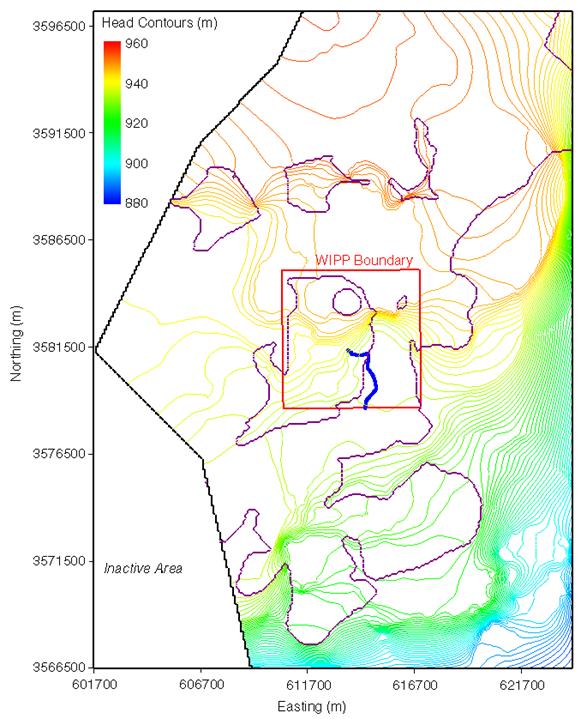
In addition to the high-T that occurs everywhere dissolution of the upper Salado has occurred, high-T zones also occur in the Culebra in the region bounded by the limit of upper Salado dissolution to the west and by the margin of where halite is present in the M2/H2 and M3/H3 intervals to the east (see Figure TFIELD-2 and Figure TFIELD-3). Fracture openness and interconnectivity in these high-T zones are controlled by a complicated history of fracturing with several episodes of cement precipitation and dissolution (Beauheim and Holt 1990; Holt 1997). No geologic metric has yet been defined that allows prediction of where fractures are filled or open, hence our knowledge of this indicator east of the Salado dissolution margin is limited to the test well locations shown in Figure TFIELD-6. Consequently, the spatial location of high-T zones between the Salado dissolution margin and the M2/H2 and M3/H3 margins is treated stochastically.
Using the hypothesized geologic controls on Culebra transmissivity, the following linear model for Y(x) = log10 T(x) was constructed:
Y(x) = β1 + β2 d(x) + β3 If (x) + β4 ID (x) (TFIELD.2)
Figure TFIELD-6. Well Locations and log10 Culebra Transmissivities
where βi (i = 1, 2, 3, 4) are regression coefficients, x is a two-dimensional location vector consisting of Universal Transverse Mercator (UTM) X and UTM Y coordinates, d(x) is the overburden thickness, If(x) is the fracture-interconnectivity indicator given in Equation (TFIELD.1) that assumes the value of 1 if fracturing and high-T have been observed at point x and 0 otherwise, and ID(x) is a dissolution indicator function that assumes the value of 1 if Salado dissolution has occurred at point x and 0 otherwise. In this model, regression coefficient β1 is the intercept value for the linear model. Coefficient β2 is the slope of Y(x)/d(x). Coefficients β3 and β4 represent adjustments to the intercept for the occurrence of interconnected fractures and Salado dissolution, respectively. Although other types of linear models could be developed, this model is consistent with the conceptual model relating transmissivity to geologic controls and can be tested using published WIPP geologic and transmissivity data. Note that the regression model does not explicitly contain terms relating Culebra transmissivity to zones where the Culebra is bounded by halite in both the M2/H2 and M3/H3 intervals because of lack of data from these areas. Therefore, it cannot be used to predict transmissivity east of the M2/H2 margin.
A linear-regression model was written using the Windows®-based program MATHCAD™ 7 Professional specifically for this application. Although other variables are input, this model requires only log10 transmissivity data from tested wells, the depth of the Culebra at those wells, and an estimate of whether dissolution of the upper Salado has or has not occurred at each location. The fracture interconnectivity indicator is defined from the log10 transmissivity data, and a Salado dissolution indicator is defined using the Salado dissolution data. These data are then used in a standard linear regression algorithm to determine the regression coefficients for Equation (TFIELD.2).
The regression coefficients for Equation (TFIELD.2) derived from this analysis are presented in Table TFIELD-1. The regression has a multiple correlation coefficient (R2) of 0.941 and a regression ANOVA F statistic of 222. The number of degrees of freedom about the regression (n) equals the number of observations (46) minus the number of parameters (4). The number of degrees of freedom due to the regression (m) equals the number of parameters (4) minus 1. With n = 42 and m = 3, the regression is significant above the 0.999 level. Residuals show no anomalous behavior. Accordingly, the regression model provides an accurate and reasonable description of the data. The fit of the regression to the log10 transmissivity data is shown in Figure TFIELD-7.
Table TFIELD-1. Regression Coefficients for Equations (TFIELD.2) and (TFIELD.3)
|
β1 |
β2 |
β3 |
β4 |
|
-5.441 |
-4.636 ´ 10-3 |
1.926 |
0.678 |
The regression model does not predict transmissivity in the regions where the Culebra is underlain by halite in the M2/H2 interval because no quantitative data were available from these regions to be used in deriving the regression. In these regions, the following modified version of the regression model of Equation (TFIELD.2) is applied:
Figure TFIELD-7. Regression Fit to Observed Culebra log10 T Data
Y(x) = β1 + β2 d(x) + β3 If (x) + β4 ID (x) + β5 IH (x) (TFIELD.3)
where IH(x) is a halite indicator function. This indicator is assigned a value of 1 in locations where halite occurs in the M2/H2 interval and 0 otherwise. The coefficient β5 is set equal to –1 so that Equation (TFIELD.3) reduces the predicted transmissivity values by one order of magnitude where halite occurs in the M2/H2 interval, to accord qualitatively with the expected transmissivity reduction discussed in Section TFIELD-3.5 of this appendix. With knowledge (or stochastic estimations) of the values of the geologic controls (e.g., Culebra depth, fracture-interconnectivity indicator, dissolution indicator, and halite indicator), Culebra transmissivity values can be predicted at unobserved locations in the WIPP Culebra model domain using Equation (TFIELD.3).
In this section, a method is developed for applying the linear regression model from Section TFIELD-3.0 of this appendix to predict Culebra transmissivity across a model domain encompassing the WIPP area. Culebra overburden thickness, Salado dissolution, and the presence or absence of halite in units bounding the Culebra can be deterministically evaluated across the WIPP region using maps constructed from subsurface data (Section TFIELD-2.0). The presence of open, interconnected fractures, however, cannot be deterministically assessed across the WIPP area using maps. A geostatistical approach, conditional indicator simulation, is used to generate 500 equiprobable realizations of zones with hydraulically significant fractures in the WIPP region. These simulations are parameterized using the frequency of occurrence of WIPP wells with hydraulically significant fractures and a fit to a variogram constructed using data from those same wells. The regression model is then applied to the entire WIPP area by:
1. Overlaying the geologic map data for Culebra overburden thickness, Salado dissolution, and the presence or absence of halite in units bounding the Culebra with each of the 500 equiprobable realizations of zones containing open, interconnected fractures
2. Sampling each grid point within the model domain to determine the overburden thickness and the indicator values for Salado dissolution, overlying or underlying halite, and fracture interconnectivity
3. Using the sampled data at each grid point with the regression model coefficients to estimate Culebra transmissivity
When applied to the 500 equiprobable realizations of zones containing open, interconnected fractures, this procedure generates 500 stochastically varying Culebra base T fields. Details about the creation of the base T fields are given in Holt and Yarbrough (2002, 2003a, 2003b).
Two principal factors were considered in selecting the boundaries for the Culebra model domain. First, model boundaries should coincide with natural groundwater divides where feasible, or be far enough from the southern portion of the WIPP site, where transport will be modeled, to have minimal influence in that area. Second, the model domain should encompass known features with the potential to affect Culebra water levels at the WIPP site (e.g., potash tailings ponds). The modeling domain selected is 22.4 kilometers (km) (13.9 miles [mi]) east-west by 30.7 km (19.1 mi) north-south, aligned with the compass directions (Figure TFIELD-6). This is the same as the domain used by LaVenue, Cauffman, and Pickens (1990) except that the current domain extends 1 km (0.62 mi) farther to the west than the 1990 domain. The modeling domain is discretized into 68,768 uniform 100 m (328 ft) by 100 m (328 ft) cells. The northern model boundary is slightly north of the northern end of Nash Draw, 12 km (7.5 mi) north of the northern WIPP site boundary and about 1 km (0.62 mi) north of Mississippi Potash Incorporated’s east tailings pile. The eastern boundary lies in a low-T region that contributes little flow to the modeling domain. The southern boundary lies 12.2 km (7.6 mi) south of the southern WIPP site boundary, 1.7 km (1.5 mi) south of our southernmost well (H-9) and far enough from the WIPP site to have little effect on transport rates on the site. The western model boundary passes through the IMC tailings pond (Laguna Uno of Hunter [1985]) due west of the WIPP site in Nash Draw. Boundary conditions assigned for the model are discussed in Section TFIELD-6.2. The coordinates of each corner of the domain are given in Table TFIELD-2, in North American Datum 27 UTM coordinates.
Table TFIELD-2. Coordinates of the Numerical Model Domain Corners
|
Domain Corner |
UTM X Coordinate (m) |
UTM Y Coordinate (m) |
|
Northeast |
624,050 |
3,597,150 |
|
Northwest |
601,650 |
3,597,150 |
|
Southeast |
624,050 |
3,566,450 |
|
Southwest |
601,650 |
3,566,450 |
To create useable data sets for conditional simulation of high-T zones and prediction of Culebra transmissivity, the geological maps described above in Section TFIELD-2.0 were imported into a geographic information systems environment and digitized. A uniform 100-m (328-ft) grid was then created over the Culebra model domain. Using the Culebra structure contour map data (Figure TFIELD-1) and surface elevation data obtained from the United States Geological Survey (USGS) National Elevation Dataset (U.S. Geological Survey 2002), an isopach map of the Culebra overburden on the 100-m (328-ft) model grid was created.
Using maps showing occurrence of halite in the units above and below the Culebra and well locations, soft data files were created for conditional indicator simulations. Transmissivity within 120 m (374 ft) of each well is assumed to be from the same population (e.g., high- or low-T reflecting open, interconnected fractures or filled (poorly interconnected) fractures, respectively), and regions where the Culebra is overlain by halite in M3/H3 or underlain by halite in M2/H2 are assumed to be low-T regions.
Using maps of Salado dissolution and the occurrence of halite in the units above and below the Culebra, 100-m (328-ft) indicator grids were created over the model domain. These indicator grids were created for regions affected by Salado dissolution, regions where the Culebra is underlain by halite in the M2/H2 interval, and a middle zone in which the Culebra is neither overlain nor underlain by halite where high-T zones occur stochastically (Figure TFIELD-8).
Excluding data where Salado dissolution occurs, Culebra transmissivity data are indicator transformed (1 for log10 transmissivity (m2/s) > -5.4, 0 otherwise). A high-T indicator variogram is then constructed for the indicator data in the region not affected by Salado dissolution using the Geostatistical Software Library (GSLIB) program GAMV (Deutsch and Journel 1998). The lag spacing for this variogram is selected to maximize variogram resolution. The resulting indicator variogram is then fit with an isotropic spherical variogram model:
Figure TFIELD-8. Zones for Indicator Grids
 (TFIELD.4)
where γ(h) is the variogram as a function of lag spacing h, s is the sill value of the indicator variogram, and l is the correlation length. This variogram model minimizes the mean squared error between the experimental and modeled variogram. The sill value was determined using:
s = P[log10 T (m2/s) > -5.4] – {P[log10 T (m2/s) > -5.4]}2 (TFIELD.5)
where P[·] is a cumulative distribution function. For the Culebra data set, excluding wells where dissolution has occurred, s = 0.201. The correlation length l was estimated to be 1,790 m (5,873 ft). No nugget effect was included in the variogram model (Figure TFIELD-9). Variogram model parameters were then used in conditional indicator simulations of Culebra high-T zones.
“Soft” indicator data were created for the indicator simulations. To ensure that no high-T regions develop in areas where halite occurs in M2/H2 or M3/H3, soft data points, indicating low-T, were placed on a 200-m (656-ft) grid east of the M2/H2 and M3/H3 salt margins. This 200-m (656-ft) grid used the original 100-m (328-ft) grid excluding every other node to assure the 200-m (656-ft) soft data grid spatially overlay the 100-m (328-ft) grid. Soft data were also specified for every 100-m (328-ft) node along the combined lines of the M2/H2 and M3/H3 salt margins.
Additional soft data were created near well locations establishing a 120-m (394-ft) buffer around each well (Figure TFIELD-10). All 100-m (328-ft) grid nodes lying within the 120-m (394-ft) buffer were selected and assigned the transmissivity attribute of the well. Because all the nodes within 120 m (394 ft) of the well and the node corresponding to the block containing the well were selected as soft data, there was duplication in the input files. Only one data point can occupy a 100-m (328-ft) grid space during a realization. Therefore, the node closest to the well was eliminated from the soft data file.
Figure TFIELD-9. High-T Indicator Model and Experimental Variograms
Figure TFIELD-10. Soft Data Around Wells
Five hundred conditional indicator simulations were generated on the 100-m (328-ft) model grid using the GSLIB program SISIM (Deutsch and Journel 1998) with Culebra high-T indicator data, soft data for regions around wells and regions where halite underlies and overlies the Culebra, and the variogram parameters. The resulting indicator simulations were used in the construction of base T fields.
The linear predictor (Equation (TFIELD.3) was used to generate 500 equally probable realizations of the transmissivity distribution in the Culebra model domain. This calculation required the regression coefficients discussed in Section TFIELD-3.8, Culebra depth data (Section TFIELD-3.2), a Salado dissolution indicator function, an indicator for where halite occurs in M2/H2, and the 500 realizations of high-T indicators discussed in Section TFIELD-4.4.
The 500 base T fields were created in five sets. Each set consists of 10 groups of 10 realizations given d##r## designations. The “d” counter ranges from 01 to 50, while the “r” counter ranges from 01 to 10. An example base T field is shown in Figure TFIELD-11. Stochastically located patches of relatively high-T (yellowish-green) can be clearly seen in the middle zone of the model domain. (Note: On black and white copy, these patches appear as the lightest shade of gray.)
Figure TFIELD-11. Example Base T Field
The base T fields described in Section TFIELD-4.5 rely on a regression model to estimate transmissivity at every location. By the nature of regression models, the estimated transmissivity values will not honor the measured transmissivity values at the measurement locations. Therefore, before using these base T fields in a flow model, they must be conditioned to the measured transmissivity values. This conditioning is performed with a Gaussian geostatistical simulation algorithm to generate a series of 500 spatially correlated residual fields where each field has a mean value of zero. These fields are conditional such that the residual value at each measurement location, when added to the value provided by the regression model (which is the same for all 500 fields), provides the known transmissivity value at that location. The result of adding the simulated residual field to the base T field is the “seed” realization.
This process is shown conceptually along a west-to-east cross section of the Culebra in Figure TFIELD-12. The upper image shows the value of the residuals at five transmissivity measurement locations across the cross section. These residuals are calculated as the observed (measured) transmissivity value minus the base field transmissivity value at the same locations. Positive residuals are where the measured transmissivity value is greater than that of the base T field. To create a T field from these residuals, there needs to be a way to tie the base field to the measured transmissivity values. This tie is accomplished by creating a spatial simulation of the residual values, a “residual field.” The middle image of Figure TFIELD-12 is an example residual field as a (red) dashed line along the cross section. This residual field is constructed through geostatistical simulation using a variogram model fit to the residual data. The residual field honors the measured residuals at their measurement locations and returns to a mean value of zero at distances far away from the measurement locations. Finally, this residual field is added to the base T field to create the seed T field. The base T field is represented by the solid (blue) line in the bottom image of Figure TFIELD-12 and the seed T field is shown by the dotted line. The seed T field corresponds to the base T field except at those locations where it must deviate to match the measured transmissivity data. The large discontinuity shown in the base T field at the bottom of Figure TFIELD-12 is due to the stochastic simulation of high-T zones within the Culebra.
A total of 46 measured transmissivity values and corresponding residual data, both in units of log10 (m2/s), are available (Table TFIELD-3). For each pair of log10 transmissivity and residual data, the well name and the easting (X) and northing (Y) UTM coordinates are also given (for multiwell hydropads, a single well’s coordinates were used).
The process of creating the residual fields is to use the residual data to generate variograms in the VarioWin software package and to then create conditional stochastic Gaussian geostatistical simulations of the residual field within the GSLIB program SGSIM (Deutsch and Journel 1998).
To use the data in a Gaussian simulation algorithm, it is first necessary to transform the distribution of the raw residual data to a standard normal distribution. This is accomplished through a process called the “normal-score transform,” where each transformed residual value is the normal score of each original datum. The normal-score transform is a relatively simple two-step process. First the cumulative frequency of each original residual value, cdf(i), is determined as:
Figure TFIELD-12. Conceptual Cross Section Showing the Updating of the Residual Field and the Base T Field into the Seed T Field
where R(i) is the rank (smallest to largest) of the ith residual value and N is the total number of data (46 in this case). Then for each cumulative frequency value, the corresponding normal-score value is calculated from the inverse of the standard normal distribution. By definition, the standard normal distribution has a mean of 0.0 and a standard deviation of 1.0. Further details of the normal-score transform process can be found in Deutsch and Journel (1998).
The two-step normal-score transformation process is conducted in Microsoft® Excel® (see details in McKenna and Hart 2003b). The resulting normal-score values are the distance from the mean as measured in standard deviations. The parameters describing the residual and normal-score transformed distributions are presented in Table TFIELD-4.
|
Table TFIELD-3. log10 Transmissivity Data Used in Inverse Calibrations |
||||
|
|
Easting |
Northing |
log10 T |
log10 T Residual |
|
AEC-7 |
621126 |
3589381 |
-6.8 |
-0.11078 |
|
CB-1 |
613191 |
3578049 |
-6.5 |
-0.32943 |
|
D-268 |
608702 |
3578877 |
-5.7 |
0.27914 |
|
DOE-1 |
615203 |
3580333 |
-4.9 |
-0.21004 |
|
DOE-2 |
613683 |
3585294 |
-4.0 |
0.69492 |
|
Engle |
614953 |
3567454 |
-4.3 |
-0.51632 |
|
ERDA-9 |
613696 |
3581958 |
-6.3 |
0.15250 |
|
H-1 |
613423 |
3581684 |
-6.0 |
0.41295 |
|
H-2c |
612666 |
3581668 |
-6.2 |
0.13594 |
|
H-3b1 |
613729 |
3580895 |
-4.7 |
-0.22131 |
|
H-4c |
612406 |
3578499 |
-6.1 |
0.05221 |
|
H-5c |
616903 |
3584802 |
-6.7 |
0.02946 |
|
H-6c |
610610 |
3584983 |
-4.4 |
-0.01524 |
|
H-7c |
608095 |
3574640 |
-2.8 |
0.39794 |
|
H-9c |
613974 |
3568234 |
-4.0 |
-0.22763 |
|
H-10b |
622975 |
3572473 |
-7.4 |
-0.01484 |
|
H-11b4 |
615301 |
3579131 |
-4.3 |
0.25314 |
|
H-12 |
617023 |
3575452 |
-6.7 |
-0.07647 |
|
H-14 |
612341 |
3580354 |
-6.5 |
-0.26934 |
|
H-15 |
615315 |
3581859 |
-6.8 |
-0.12631 |
|
H-16 |
613369 |
3582212 |
-6.1 |
0.34962 |
|
H-17 |
615718 |
3577513 |
-6.6 |
-0.14310 |
|
H-18 |
612264 |
3583166 |
-5.7 |
0.73159 |
|
H-19b0 |
614514 |
3580716 |
-5.2 |
-0.62242 |
|
P-14 |
609084 |
3581976 |
-3.5 |
0.16212 |
|
P-15 |
610624 |
3578747 |
-7.0 |
-0.95938 |
|
P-17 |
613926 |
3577466 |
-6.0 |
0.24762 |
|
USGS-1 |
606462 |
3569459 |
-3.3 |
0.28998 |
|
WIPP-12 |
613710 |
3583524 |
-7.0 |
-0.39627 |
|
WIPP-13 |
612644 |
3584247 |
-4.1 |
0.42180 |
|
WIPP-18 |
613735 |
3583179 |
-6.5 |
0.06840 |
|
WIPP-19 |
613739 |
3582782 |
-6.2 |
0.32598 |
|
WIPP-21 |
613743 |
3582319 |
-6.6 |
-0.11148 |
|
WIPP-22 |
613739 |
3582653 |
-6.4 |
0.10549 |
|
Table TFIELD-3. log10 Transmissivity Data Used in Inverse Calibrations (Continued) |
||||
|
Well |
Easting |
Northing |
log10 T |
log10 T Residual |
|
WIPP-25 |
606385 |
3584028 |
-3.5 |
-0.01378 |
|
WIPP-26 |
604014 |
3581162 |
-2.9 |
0.21598 |
|
WIPP-27 |
604426 |
3593079 |
-3.3 |
-0.03209 |
|
WIPP-28 |
611266 |
3594680 |
-3.6 |
-0.15124 |
|
WIPP-29 |
596981 |
3578694 |
-3.0 |
-0.12497 |
|
WIPP-30 |
613721 |
3589701 |
-6.7 |
-0.35131 |
|
WQSP-1 |
612561 |
3583427 |
-4.5 |
0.01540 |
|
WQSP-2 |
613776 |
3583973 |
-4.7 |
-0.02729 |
|
WQSP-3 |
614686 |
3583518 |
-6.8 |
-0.15139 |
|
WQSP-4 |
614728 |
3580766 |
-4.9 |
-0.28895 |
|
WQSP-5 |
613668 |
3580353 |
-5.9 |
0.47178 |
|
WQSP-6 |
612605 |
3580736 |
-6.6 |
-0.32261 |
Table TFIELD-4. Statistical Parameters Describing the Distributions of the Raw and Normal-Score Transformed Residual Data
|
Parameter |
Raw Residual |
Normal-Score Transformed Residual Data |
|
Mean |
0.000 |
0.000 |
|
Median |
-0.015 |
0.000 |
|
Standard Deviation |
0.330 |
0.997 |
|
Minimum |
-0.959 |
-2.295 |
|
Maximum |
0.732 |
2.295 |
The omnidirectional variogram is calculated with a 250-m (820-ft) lag spacing. The experimental variogram is shown in Figure TFIELD-13. The model fit to this experimental variogram is Gaussian with a nugget of 0.2, a sill of 0.8, and a range of 1,050 m (3,445 ft). The sum of the nugget and sill values is constrained to equal the theoretical variance of 1.0 by the sgsim software that is used to create the spatially correlated residual fields.
The variogram parameters for the normal-score transformed residuals are used directly in the sgsim program to create 500 conditional realizations of the residual field. Each of these 500 residual fields is used as an initial residual field and each one is assigned to an individual base T field. An example of a realization of the residual field and its combination with a base T field is shown in Figure TFIELD-14. From Figure TFIELD-14, the effect of the residual field on the base T field can be seen. The residual field perturbs the transmissivities to match the measured transmissivities at the well locations. The discrete features that are part of the original base
Figure TFIELD-13. Omnidirectional Variogram Model Fit to the Experimental Variogram of the Transmissivity Residuals
Figure TFIELD-14. An Example of the Creation
of a Seed T Field.
The Base T Field (Left Image) is Combined with the Initial
Residual Field Created Through Geostatistical Simulation (Center
Image) to Produce the Seed T Field (Right Image). That
Field is Then Used as the Initial Field for the First Iteration
of the Inverse Calibration Procedure. All Three Color
Scales Denote the log10 Transmissivity
(m2/s) Value.
T field (e.g., high-T zones in the middle of the domain) are retained when the residual field is added to the base field, although transmissivity values within those features may be altered to a degree.
A number of distributed locations within the modeling domain are selected and designated as “pilot points.” PEST adjusts the transmissivity value at each of these pilot points to achieve a better match between the groundwater flow model results and the observed steady-state and transient head data. The adjustments in transmissivity at each pilot point cannot be made independently of surrounding transmissivity values and, therefore, these surrounding transmissivity values must be updated in a manner consistent with the change made at the pilot point. This updating is done by applying a change at each of the surrounding points that is a weighted fraction of the change made at the pilot point. The weights are calculated from the residual variogram.
These updates are necessary to create a final T field that honors all observed transmissivity measurements and matches the observed heads when used as input to a groundwater flow model. Therefore, it is also necessary to calculate and model a variogram on the raw, not normal-score transformed residuals for use in this kriging process.
This variogram was also calculated with a 250-m (820-ft) lag and is omnidirectional. A doubly nested spherical variogram model was fit to the experimental variogram. The variogram parameters are a nugget of 0.008, a first sill and range of 0.033 and 500 m (1,640 ft), respectively, and a second sill and range of 0.067 and 1,500 m (4,921 ft), respectively (Figure TFIELD-15).
Figure TFIELD-15. Experimental and Model Variograms for the Raw-Space (Not Normal-Score Transformed) Transmissivity Residual Data
This section presents details on the modeling approach used to calibrate the T fields to both the 2000 steady-state heads and 1,332 transient drawdown measurements. This section is divided into the following subsections:
1. Assumptions made in the modeling and the implications of these assumptions are provided. (Section TFIELD-6.1)
2. The initial heads used for each calibration are estimated at each location in the domain using the heads measured in 2000 using kriging and accounting for the regional trend in the head values. (Section TFIELD-6.2)
3. The initial heads are used to assign fixed-head boundaries to three sides of the model. The fourth side, the western edge, is set as a no-flow boundary for the model. (Section TFIELD-6.3)
4. The transient head observations for each hydraulic test and each observation well are selected from the database. These heads are shown as a function of time for each hydraulic test. (Section TFIELD-6.4)
5. The spatial and temporal discretization of the model domain are presented. (Section TFIELD-6.5 and Section TFIELD-6.6)
6. The transient head observations are given relative weights based on the inverse of the maximum observed drawdown in each hydraulic test. The relative weights assigned to the steady-state observations are also discussed. (Section TFIELD-6.7)
7. The locations of the adjustable pilot points are determined using a combination of approaches. (Section TFIELD-6.8)
All of these steps can be considered as preprocessing aspects of the stochastic inverse calibration procedure. The actual calibrations are done using an iterative coupling of the MODFLOW-2000 and PEST codes. The details of this process are covered in McKenna and Hart (2003a, 2003b), and are briefly summarized in Section TFIELD-6.9.
The major assumptions that apply to this set of model calculations are as follows.
1. The boundary conditions along the model domain boundary are known and do not change over the time frame of the model. This assumption applies to both the no-flow boundary along the western edge of the domain as well as to the fixed-head boundaries that were created to be consistent with the 2000 head measurements in the model domain. Implicit in this assumption is that the fixed-head boundary conditions do not have a significant impact on the transient tests that were simulated in the interior of the model at times other than the 2000 period.
2. The fracture permeability of the Culebra can be adequately modeled as a continuum at the 100-m (328-ft) ´ 100-m (328-ft) grid block scale and the measured transmissivity values used to condition the model are representative of the transmissivity in the 100-m (328-ft) ´ 100-m (328-ft) grid block in which the well test was performed. Implicit in this assumption is the prior assumption that the hydraulic test interpretations were done correctly and used the correct conceptual model.
3. Variable fluid densities in the Culebra can be adequately represented by casting the numerical solution in terms of freshwater head. Davies (1989) investigated the effects of variable fluid density on the directions of flow calculated in the Culebra using a freshwater-head approach. As the Culebra flow system was conceptualized and modeled by Davies, most of the water flowing in the Culebra in the vicinity of the WIPP site ultimately discharged to the Pecos River southwest of WIPP. When variable fluid density was taken into account, the only locations within the model domain where the flow direction changed by more than 10 degrees were regions 1.1 to 14.3 km (0.7 to 8.9 mi) south of the WIPP site, where the flow direction shifted as much as 70 degrees to the east toward a more downdip direction (but still primarily to the south) (Davies, 1989, Figure 35 and Figure 36). As currently conceptualized, flow in the Culebra in the vicinity of WIPP does not discharge to the Pecos to the southwest, but instead goes to the southsoutheast toward the Paduca oilfield where extensive dissolution of the Salado and collapse of the Culebra has occurred (see Figure TFIELD-1). Hence, taking variable fluid density into account would have little effect on the flow direction.
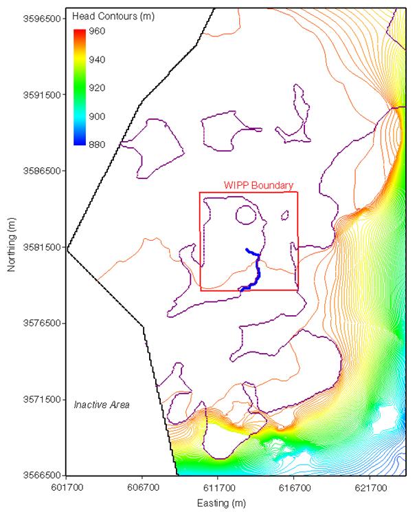
A set of initial head values was estimated across the flow model domain based on water-level measurements made in late 2000 (Beauheim 2002b). The water-level measurements were converted to freshwater heads using fluid-density data collected from pressure-density surveys performed in the wells and/or from water-quality sampling. The head values estimated at the cells in the interior of the domain were used as initial values of the heads and were subsequently updated by the groundwater flow model until the final solution was achieved. The head values estimated for the fixed-head cells along the north, east, and south boundaries of the model domain remained constant for the groundwater flow calculation. The estimation of the initial and boundary heads was done by kriging. Observed heads both within and outside of the flow model domain (Figure TFIELD-16) were used in the kriging process.
Kriging is a geostatistical estimation technique that uses a variogram model to estimate values of a sampled property at unsampled locations. Kriging is designed for the estimation of stationary fields (see Goovaerts 1997); however, the available head data show a significant trend (nonstationary behavior) from high head in the northern part of the domain to low head in the southern part of the domain. This behavior is typical of groundwater head values measured across a large area with a head gradient. To use kriging with this type of nonstationary data, a Gaussian polynomial function is fit to the data, and the differences between the polynomial and the measured data (the “residuals”) are calculated and a variogram of the residuals is constructed. This variogram and a kriging algorithm are then used to estimate the value of the residual at all locations within a domain. The final step in the process is to add the trend from the previously defined polynomial to the estimated residuals to get the final head estimates. This head estimation process is similar to that used in the Culebra calculations done for the Compliance Certification Application (CCA, U.S. Department of Energy 1996) (Lavenue 1996).
Figure TFIELD-16. Locations and Values of the 2000 Head Measurements Considered in the Steady-State Calibrations. The Approximate Extent of the Numerical Model Domain is Shown by the Black Rectangle in the Image.
The available head data from late 2000, comprising 37 measurements, are listed in Table TFIELD-5. In general, these head measurements show a trend from high head in the north to low head in the south. The trend was modeled with a bivariate Gaussian function. The use of this Gaussian function with five estimated parameters allows considerable flexibility in the shape of the trend that can be fit through the observed data. The value of the Gaussian function, Z, is:
where X0 and Y0 are the coordinates of the center of the function and b and c are the standard deviations of the function in the X (east-west) and Y (north-south) directions, respectively. The parameter a controls the height of the function. The Gaussian function was fit to the data using the regression wizard tool in the SigmaPlot® 2001 graphing software. The parameters estimated for the Gaussian function are presented in Table TFIELD-6. The fit of the Gaussian trend surface to the 2000 heads is shown in Figure TFIELD-17. The locations and values of the residuals (observed value–trend surface estimate) are shown in Figure TFIELD-18.
Table TFIELD-5. Well Names and Locations of the 37 Head Measurements Obtained in Late 2000 Used to Define Boundary and Initial Heads
|
Well |
UTM X (Easting) (m) |
UTM Y (Northing) (m) |
2000 Freshwater Head (m amsl) |
|
AEC-7 |
621126 |
3589381 |
933.19 |
|
DOE-1 |
615203 |
3580333 |
916.55 |
|
DOE-2 |
613683 |
3585294 |
940.03 |
|
ERDA-9 |
613696 |
3581958 |
921.59 |
|
H-1 |
613423 |
3581684 |
927.19 |
|
H-2b2 |
612661 |
3581649 |
926.62 |
|
H-3b2 |
613701 |
3580906 |
917.16 |
|
H-4b |
612380 |
3578483 |
915.55 |
|
H-5b |
616872 |
3584801 |
936.26 |
|
H-6b |
610594 |
3585008 |
934.20 |
|
H-7b1 |
608124 |
3574648 |
913.86 |
|
H-9b |
613989 |
3568261 |
911.57 |
|
H-11b4 |
615301 |
3579131 |
915.47 |
|
H-12 |
617023 |
3575452 |
914.66 |
|
H-14 |
612341 |
3580354 |
920.24 |
|
H-15 |
615315 |
3581859 |
919.87 |
|
H-17 |
615718 |
3577513 |
915.37 |
|
H-18 |
612264 |
3583166 |
937.22 |
|
H-19b0 |
614514 |
3580716 |
917.13 |
|
P-17 |
613926 |
3577466 |
915.20 |
|
WIPP-12 |
613710 |
3583524 |
935.30 |
|
WIPP-13 |
612644 |
3584247 |
935.17 |
|
WIPP-18 |
613735 |
3583179 |
936.08 |
|
WIPP-19 |
613739 |
3582782 |
932.66 |
|
WIPP-21 |
613743 |
3582319 |
927.00 |
|
WIPP-22 |
613739 |
3582653 |
930.96 |
|
WIPP-25 |
606385 |
3584028 |
932.70 |
|
WIPP-26 |
604014 |
3581162 |
921.06 |
|
WIPP-27 |
604426 |
3593079 |
941.01 |
|
WIPP-29 |
596981 |
3578701 |
905.36 |
|
WIPP-30 |
613721 |
3589701 |
936.88 |
|
WQSP-1 |
612561 |
3583427 |
935.64 |
|
WQSP-2 |
613776 |
3583973 |
938.82 |
|
WQSP-3 |
614686 |
3583518 |
935.89 |
|
WQSP-4 |
614728 |
3580766 |
917.49 |
|
WQSP-5 |
613668 |
3580353 |
917.22 |
|
WQSP-6 |
612605 |
3580736 |
920.02 |
Table TFIELD-6. Parameters for the Gaussian Trend Surface Model Fit to the 2000 Heads
|
Trend Surface Parameters |
Value |
|
X0 |
611011.89 |
|
Y0 |
3780891.50 |
|
a |
1134.61 |
|
b |
73559.35 |
|
c |
313474.40 |
Figure TFIELD-17. Gaussian Trend Surface Fit to the 2000 Observed Heads
The next step in estimating the initial head values is to calculate an experimental variogram for each set of residuals and then fit a variogram model to each experimental variogram. Due to the rather limited number of data points, anisotropy in the spatial correlation of the residuals was not
examined and an omnidirectional variogram was calculated. These calculations were done using the VARIOWIN (version 2.21) software (Pannatier 1996). The Gaussian variogram model is:
Figure TFIELD-18. Locations and Values of the Residuals Between the Gaussian Trend Surface Model and the Observed Head Data. The Approximate Boundary of the Flow Model is Shown as a Black Rectangle in the Image.
where C is the sill of the variogram, h is the distance between any two samples, or the lag spacing, and a is the practical range of the variogram, or the distance at which the model reaches 95 percent (%) of the value of C. In addition to the sill and range, the variogram model may also have a nonzero intercept with the gamma (Y) axis of the variogram plot known as the nugget. Due to numerical instabilities in the kriging process associated with the Gaussian model without a nugget value, a small nugget was used in fitting each of the variogram models. The model variogram was fit to the experimental data (Figure TFIELD-19) and the parameters of this model are given in Table TFIELD-7.
The experimental variogram calculated on the 2000 data in Figure TFIELD-19 shows a number of points between lags 2,000 and 7,000 m (1.25 and 4.25 mi) that are above the variance of the data set (the horizontal dashed line). This behavior indicates that the Gaussian trend surface model used to calculate the residuals from the measured data did not remove the entire trend inherent in the observed data. A higher order trend surface model could be applied to these data to remove more of the trend, but the Gaussian trend surface model provides a reasonable estimate of the trend in the data.
Figure TFIELD-19. Omnidirectional Experimental (Straight-Line Segments) and Model Variograms of the Head Residuals (Curves) for the 2000 Heads. The Numbers Indicate the Number of Pairs of Values That Were Used to Calculate Each Point and the Horizontal Dashed Line Denotes the Variance of the Residual Data Set.
Table TFIELD-7. Model Variogram Parameters for the Head Residuals
|
Parameter |
Value |
|
Sill |
22 |
|
Range (meters) |
3000 |
|
Nugget |
4.5 |
|
Number of Data |
37 |
The GSLIB kriging program KT3D (Deutsch and Journel 1998) was used to estimate the residual values at all points on the grid within the model domain. The Gaussian trend surface was then added to the estimated residual values to produce the final estimates of the initial head field.
Two types of boundary conditions were specified in MODFLOW-2000: constant-head and no-flow. Constant-head conditions were assigned along the eastern boundary of the model domain, and along the central and eastern portions of the northern and southern boundaries. Values of these heads were obtained from the kriged initial head field. The western model boundary passes through the Mosaic Potash Carlsbad tailings pond (Laguna Uno) due west of the WIPP site in Nash Draw. A no-flow boundary (a flow line) is specified in the model from this tailings pond up the axis of Nash Draw to the northeast, reflecting the concept that groundwater flows down the axis of Nash Draw, forming a groundwater divide. Similarly, another no-flow boundary is specified from the tailings pond down the axis of the southeastern arm of Nash Draw to the southern model boundary, coinciding with a flow line in the regional modeling of Corbet and Knupp (1996). Thus, the northwestern and southwestern corners of the modeling domain are specified as inactive cells in MODFLOW-2000. The initial (starting) head field is shown in Figure TFIELD-20 and the head values along each boundary of the model domain are shown in Figure TFIELD-21 and Figure TFIELD-22.
Figure TFIELD-20. Map of Initial Heads Created Through Kriging and Used to Assign Fixed-Head Boundary Conditions
Figure TFIELD-21. Values of Fixed Heads Along the Eastern Boundary of the Model Domain
Figure TFIELD-22. Values of Fixed Heads Along the Northern and Southern Boundaries of the Model Domain. Note That Not All Locations Along the Boundaries are Active Cells.
In addition to being used to generate an initial head distribution, the water-level measurements made in 35 wells within the model domain during late 2000 were also used in steady-state model calibration. (Note that Table TFIELD-5 includes data from two wells–WIPP-27 and WIPP-29–that were used to define model boundary conditions but are outside the area of calibration).
The transient observation data used for the transient calibrations were taken from a number of different sources listed in Beauheim and Fox (2003). Responses to seven different hydraulic tests were employed in the transient portion of the calibration (Table TFIELD-8). Hydraulic responses for each of the 7 tests were monitored in 3 to 10 different observation wells depending on the hydraulic test.
A major change in the calibration data set from the CCA calculations is the exclusion of the hydraulic responses to the excavation of the exploratory (now salt) and ventilation (now waste) shafts in the current calibration. The responses to the shaft excavations were excluded because:
1. Only two wells (H-1 and H-3) responded directly to the shaft excavations and the areas between the shafts and these wells are stressed by other hydraulic tests that are included in the calibration data set (H-3b2, WIPP-13, and H-19b0).
2. It was difficult to model both the flux and pressure changes accurately during the excavation of the shafts with MODFLOW-2000. This difficulty is due to both the finite-difference discretization of MODFLOW-2000 that requires each shaft to be modeled as a complete model cell and some limitations of the data set.
3. The long-term effects of the shafts on site-wide water levels were important for the CCA modeling because that modeling sought to replicate heads over time. In the current CRA 2004 calibration effort, shaft effects are not important because drawdowns resulting from specific hydraulic tests are used as the calibration targets and shaft effects can be considered as second-order compared to the effects of the hydraulic tests that are simulated.
A small amount of processing of the observed data was necessary prior to using it in the calibration process. This processing included selecting the data values that would be used in the calibration procedure from the often voluminous measurements of head. These data were chosen to provide an adequate description of the transient observations at each observation well across the response time without making the modeling too computationally burdensome in terms of the temporal discretization necessary to model responses to these observations. Scientific judgment was used in selecting these data points. This selection process resulted in a total of 1,332 observations for use in the transient calibration.
Additionally, the modeling of the pressure data is done here in terms of drawdown. Therefore, the value of drawdown at the start of any transient test must be zero. A separate Perl script was written to normalize each set of observed heads to a zero value reference at the start of the test with the exception of the H-3 test that is only preceded by the steady-state simulation. The calculations are such that the resulting drawdown values are positive.
Table TFIELD-8. Transient Hydraulic Test and Observation Wells for the Drawdown Data
|
Stress Point |
Observation Well |
Observation Start |
Observation End |
Observation Type |
|
H-3b2 |
DOE-1 |
10/15/1985 |
3/18/1986 |
Drawdown |
|
WIPP-13 |
DOE-2 |
1/12/1987 |
5/15/1987 |
Drawdown |
|
P-14 |
D-268 |
2/14/1989 |
3/7/1989 |
Drawdown |
|
H-11b1 |
H-4b |
2/7/1996 |
12/11/1996 |
Drawdown |
|
H-19b0 |
DOE-1 |
12/15/1995 |
12/10/1996 |
Drawdown |
|
WQSP-1 |
H-18 |
1/25/1996 |
2/20/1996 |
Drawdown |
|
WQSP-2 |
DOE-2 |
2/20/1996 |
3/28/1996 |
Drawdown |
In addition to normalizing the measured head data, some of the tests produced negative drawdown values when normalized. These negative results are due to some of the observations having heads greater than the reference value. This occurs due to some hydraulic tests that were conducted at earlier times in the Culebra but were not included in the numerical model. If the drawdowns from one of these previous tests are still recovering to zero at the start of a simulation, they can cause negative drawdowns in the simulation as the recovery continues. Most of these effects were addressed through trend removal in initial data processing (Beauheim and Fox 2003) but some residual effects remain.
The resultant transient calibration points are shown in Figure TFIELD-23 through Figure TFIELD-36. These sets of figures show the location of each hydraulic test and the locations of the observation wells for that test within the model domain and the time series of drawdown values for each observation well. The values of drawdown are in meters where a positive drawdown indicates a decrease in the pressure within the well relative to the pressure before the start of the pumping (negative drawdown values indicate rises in the water level). For the Water Quality Sampling Program (WQSP)-1 and WQSP-2 tests, well WQSP-3 showed no response. These results are used in the calibration process by setting the observed drawdown values to zero for WQSP-3. The maps in Figure TFIELD-23 through Figure TFIELD-35 also show the locations of the pilot points used in the calibration (these are discussed later).
The flow model was discretized into 68,768 regular, orthogonal cells each of which represents 100 m (328 ft) ´ 100 m (328 ft). A constant Culebra thickness of 7.75 m (25.4 ft) was used (the CCA, Appendix TFIELD). The 100-m (328-ft) grid discretization was selected to make the finite-difference grid cell sizes considerably finer, on average, than those used in the CCA calculations, but still computationally tractable. In the CCA calculations, a telescoping finite-difference grid was used with the smallest cell being 100 m (328 ft) ´ 100 m (328 ft) near the center of the domain. The largest cells in the CCA flow model grid were 800 m (2,625 ft) ´ 800 m (2,625 ft) near the edges of the domain (Lavenue 1996).
The cells in the model domain were assigned elevations based on the digitized version of Figure TFIELD-1. Of the 68,768 cells (224 east-west by 307 north-south), 14,999 (21.8%) lie to the west of the no-flow boundary, so the total number of active cells in the model is 53,769. This number is nearly a factor of five larger than the 10,800 (108 ´ 100) cells used in the CCA calculations.
The time period of nearly 11 years and 2 months covered by the transient modeling began October 15, 1985, and ended December 11, 1996. Additionally, a single steady-state calculation was run prior to the transient modeling. The length of this steady-state time period and the date at which it occurs were arbitrarily set to one day (86,400 s) occurring from October 14, 1985, to October 15, 1985. These steady-state heads were measured in the year 2000 and were only set to these October dates to provide a steady-state solution prior to the start of any transient hydraulic events. The responses to the transient events were defined by the amount of drawdown relative to the initial steady-state solution. The discretization of this time interval was dictated by the pumping history of the different wells used in the hydraulic testing and consideration of the additional computational burden required for increasingly fine time discretization.
Figure TFIELD-23. Locations of the H-3b2 Hydraulic Test Well and Observation Wells
Figure TFIELD-24. Observed Drawdowns for the H-3b2 Hydraulic Test
The groundwater flow model, MODFLOW-2000, allows for the discretization of time into both “stress periods” and “time steps.” A stress period is a length of time over which the boundary conditions and internal stresses on the system are constant. Even though these stresses are constant, this does not mean that the flow system is necessarily at steady state during the stress period. A time step is a subdivision of a stress period. System information such as the head or drawdown values is only calculated at the specified time steps. Each stress period must contain at least one time step. MODFLOW-2000 allows for the specification of the stress period length, the number of time steps in the stress period, and a time step multiplier. The time step multiplier increases the time between successive time steps geometrically. This geometric progression provides a nearly ideal time discretization for the start of a pumping or recovery period. To save on computational costs associated with calculating head/drawdown at each time step and with writing out the heads/drawdowns, the number of time steps in the model was kept to the minimum number possible that still adequately simulated the hydraulic tests. The time discretization in MODFLOW-2000 resulted in modeled heads calculated at times that sometimes differed from the observation times. For this situation, the PEST utility mod2obs was used to interpolate the head, or drawdown, values in time from the simulation times to the observation times.
A summary of the time discretization is given in Table TFIELD-9. There are five separate MODFLOW-2000 simulations for each complete forward simulation of the transient events. Each separate call to MODFLOW-2000 has its own set of input and output files. In Table TFIELD-9, each call to MODFLOW-2000 is separated by a horizontal black line. The first call is the steady-state simulation. The second, third, and fourth calls to MODFLOW-2000 (H-3, WIPP-13, and P-14) are all similar in that a single well was pumped. For the H-3 and WIPP-13 calls, there were a total of three stress periods. In the first stress period, the well was pumping at a constant rate; in the second stress period, the pumped well was inactive and heads were recovering after the cessation of pumping; and the final stress period was simply a long time of no pumping activity used to advance the simulation time to be consistent with the calendar time. The first two stress periods were discretized using eight time steps and the final stress period with no pumping activity was discretized using the minimum possible number of time steps—one.
Figure TFIELD-25. Locations of the WIPP-13 Hydraulic Test Well and Observation Wells
Figure TFIELD-26.
Observed Drawdowns for the WIPP-13 Hydraulic Test.
Note the Change in the Scale of the Y-Axis from the Upper to the
Lower Image.
The final MODFLOW-2000 call, the H-19 call, was considerably more complicated than the earlier calls to MODFLOW-2000 and simulated the hydraulic conditions during the H-11, H-19, WQSP-1, and WQSP-2 hydraulic tests. This final call contained 17 stress periods with as many as 3 different wells pumping during any single stress period. The pumping rates of the different wells in this call to MODFLOW-2000 and the stress periods are shown as a function of time in Figure TFIELD-37. The first six stress periods in this call simulated pumping in the H-19 and H-11 wells without any observations (Table TFIELD-9). These pumping periods were added to the model solely to account for the effects of these tests in observations of later hydraulic tests and, therefore, these tests could be modeled with a single time step. The pumping rates shown in Figure TFIELD-37 are given as negative values to indicate the removal of water from the Culebra following the convention used in MODFLOW-2000.
Figure TFIELD-27. Locations of the P-14 Hydraulic Test Well and Observation Wells
Figure TFIELD-28. Observed Drawdowns for the P-14 Hydraulic Test
The MODFLOW-2000 simulations could be done using a single call to MODFLOW-2000, but five separate calls were used here. Each of the five calls created separate binary output files of drawdown and head that were much smaller and easier to manage than a single output file would have been. Additionally, the simulated drawdowns at the start of each transient test must be zero (no drawdown prior to pumping). Because MODFLOW-2000 uses the resulting drawdowns and heads from the previous stress period as input to the next stress period, a single simulation would not necessarily start each transient test with zero drawdowns. Calling MODFLOW-2000 five times allowed the initial drawdowns to be reset to zero each time using shell scripts. The heads simulated at the end of the final time step in each MODFLOW-2000 call were used as the initial heads for the next call. The results of all five calls were combined to produce the 1332 model predictions prior to comparing them to the 1332 selected observation data, thus ensuring that all steady-state and transient data were used simultaneously in the inverse calibration procedure.
The observed data for each response to each transient hydraulic test are weighted to take into account the differences in the responses across the different tests. The weights are calculated as the inverse of the maximum observed drawdown for each hydraulic test. This weighting scheme applies relatively less weight to tests with large drawdowns and relatively more weight to tests with smaller responses. This weighting scheme was used so that the overall calibration was not dominated by trying to reduce the very large residuals that may occur at a few of the observation locations with very large drawdowns. Under this weighting scheme, two tests that are both fit by the model to within 50% of the observed drawdown values would be given equal consideration in the calculation of the overall objective function even though one test may have an observed maximum drawdown of 10 m (33 ft) and the other a maximum observed drawdown of 0.10 m (0.33 ft).
Figure TFIELD-29. Locations of the WQSP-1 Hydraulic Test Well and Observation Wells
Figure TFIELD-30. Observed Drawdowns for the WQSP-1 Hydraulic Test
The weights assigned in this manner ranged from 0.052 to 20.19. The observed absence of a hydraulic response at WQSP-3 to pumping at WQSP-1 and WQSP-2 was also included in the calibration process by inserting measurements of zero drawdown that were given an arbitrarily high weight of 20. Through trial and error using the root mean squared error (RMSE) criterion of how well the modeled steady-state heads fit the observed steady-state heads, a weight of 2.273 was assigned to the 35 steady-state observations. This weight is near that of the average of all the weights assigned to the transient events and was found to be adequate to provide acceptable steady-state matches. It is noted that the steady-state data provide measurements of head while all of the transient events provide measurements of drawdown. However, the weights were applied to the residuals between the observed and modeled aquifer responses and because both heads and drawdowns are measured in meters, there was no need to adjust the weights to account for different measurement units.
The number of measurements used for calibrations that were made at individual wells during individual tests ranged from 6 to 104, and the number of measurements used for calibration that were made at all wells during a single test ranged from 64 to 410. This means that different well responses and different tests carried different cumulative weights. The spatially broadest sampling of transient data possible was used in an effort to get transient coverage of as much of the modeling domain as possible. In those areas where no transient data are available, the calibration is dominated by fitting the model to the steady-state measurements. The greatest coverage of transient data is within the boundaries of the WIPP site, which is also the area of most significance for radionuclide transport.
The maximum observed drawdown, the weight assigned to all the observed test values for each test, and the total number of observations for each observation well are given in Table TFIELD-10. In a few cases, weights were increased to obtain better fits, or decreased due to high degrees of noise in the data.
Figure TFIELD-31. Locations of the WQSP-2 Hydraulic Test Well and Observation Wells
Figure TFIELD-32. Observed Drawdowns from the WQSP-2 Hydraulic Test
A major development in the field of stochastic inverse modeling that has occurred since the T fields were constructed for the CCA in 1996 is that inverse techniques are now capable of simultaneously determining optimal transmissivity values at a large number of pilot points. In the T fields constructed for the CCA, pilot points were added one at a time and each point was calibrated prior to the addition of the next pilot point. Furthermore, the total number of pilot points was limited to less than or equal to the total number of transmissivity observations to avoid numerical instabilities in the solution of the inverse problem. With the techniques now available and implemented in PEST, it is possible to use many more pilot points than there are transmissivity observations and to calibrate these pilot points simultaneously.
The pilot-point locations were chosen using a combination of a regular grid approach and deviations from that grid to accommodate specific pumping- and observation-well locations (Figure TFIELD-38). The goal in these deviations from the regular grid was to put at least one pilot point between each pumping well and each of its observation wells. Details of the pilot-point locations relative to the pumping and observation wells in the WIPP site area are shown in Figure TFIELD-39. This combined approach of a regular grid with specific deviations from that grid follows the guidelines for pilot-point placement put forth by John Doherty (the author of PEST 2003) (Doherty 2002) as Appendix 1 in the work of McKenna and Hart (2003a). Pilot points located at the transmissivity measurement locations were held as fixed values during the optimization (fixed pilot points shown as magenta squares in Figure TFIELD-38). The variable pilot points (dark blue diamonds in Figure TFIELD-38) are those where the transmissivity value was adjusted during the calibration procedure. A total of 43 fixed and 100 variable pilot points was used in the T-field calibration process. The zone option in PEST was employed to limit the influence of pilot points in any one zone (e.g., high-T or low-T) to adjusting only locations that are in the same zone.
Figure TFIELD-33. Locations of the H-11 Hydraulic Test Well and Observation Wells
Figure TFIELD-34. Observed Drawdowns for the H-11 Hydraulic Test
The variogram model for the residuals between the transmissivity measurements and the base field has a range of 1,050 m (3,445 ft). Because the pilot-point approach to calibration uses this range as a radius of influence, locations of the adjustable pilot points were as much as possible set to be at least 1,050 m (3,445 ft) away from other pilot points (adjustable or fixed). For maximum impact, all pilot points should be at least 2,100 m (6,890 ft) away from any other pilot point but, given the existing well geometry, this distance was not always achievable.
The seed realizations are input to the inverse model using the pilot-point method. The seed realizations are calibrated to the steady-state and transient head measurements. The residuals and the T-field calculations are done in log10 space so that a unit change in the residual equates to a one order of magnitude change in the value of transmissivity. The initial values of the pilot points are equal to the value of the initial residual field at each pilot-point location. The pilot points are constrained to have a maximum perturbation of ±3.0 from the initial value except for those pilot points within the high-T zone in Nash Draw (Figure TFIELD-11) and the low-T zone on the eastern side of the model domain that are limited to perturbations of ±1.0. These limits are employed to maintain the influence of the geologic conceptual model on the calibrated T fields.
Figure TFIELD-11 is updated as Figure TFIELD-40 to show, conceptually, how the addition of two pilot points along the cross section can modify the residual field and then update the T field. The pilot points are shown as the open circles in Figure TFIELD-40 and are used to modify the residual field before it is added to the base T field. Compare the shape of the dashed red and blue lines in Figure TFIELD-40 to the same lines in Figure TFIELD-11. The values of the residuals at the observation points are held fixed so any adjacent pilot points cannot modify them.
Figure TFIELD-35. Locations of the H-19 Hydraulic Test Well and Observation Wells
Figure TFIELD-36. Observed Drawdowns From the H-19 Hydraulic Test
At the heart of the calibration process is the iterative adjustment of the residual field at the pilot points by PEST and the subsequent updates of the residual field at the locations surrounding the pilot points based on the shape of the variogram modeled on the raw residuals. The updated residual field is then combined with the base T field (see Figure TFIELD-18) and then used in MODFLOW-2000 to calculate the current set of modeled heads. These modeled heads are then input to PEST for the next iteration.
The objective function minimized by PEST (phi) is a combination of the weighted sum of the squared residuals between the measured and observed steady-state head data, the weighted sum of the squared residuals between the measured and observed transient drawdown data, and the weighted sum of the squared differences in the estimated transmissivity value between pairs of pilot points.
Table TFIELD-9. Discretization of Time into 29 Stress Periods and 127 Time Steps with Pumping Well Names and Pumping Rates
|
Event Name |
Global Stress Period No. |
Internal Stress Period No. |
Stress Period Length (s) |
No. of Time Steps |
Start Date |
Stop Date |
Pumping Well(s) |
Pumping Rate(s) (m3/s) |
|
Steady |
1 |
1 |
86400 |
1 |
10/14/859:00 |
10/15/859:00 |
0 |
0 |
|
H-3 |
2 |
1 |
5356800 |
8 |
10/15/859:00 |
12/16/859:00 |
H-3 |
3.03E-04 |
|
WIPP-13 |
5 |
1 |
3110400 |
8 |
1/12/879:00 |
2/17/879:00 |
WIPP-13 |
1.89E-03 |
|
P-14 |
8 |
1 |
44928 |
3 |
2/14/899:01 |
2/14/8921:29 |
P-14 |
3.92E-03 |
|
H-19 |
13 |
1 |
148860 |
1 |
4/24/9519:42 |
4/26/95 13:03 |
H-19b0 |
2.26E-04 |
Figure TFIELD-37.
Temporal Discretization and Pumping Rates for the Fifth Call to
MODFLOW-2000.
A Total of 17 Stress Periods (SPs) are Used to Discretize this
Model Call.
Table TFIELD-10. Observation Weights for Each of the Observation Wells
|
Test Well Observation Well |
Maximum Drawdown (m) |
Weight |
Number of Observations |
|
Steady |
NA |
2.273 |
35 |
|
H3-DOE1 |
5.426 |
0.184 |
57 |
|
W13-DOE2 |
12.138 |
0.082 |
104 |
|
P14-D268 |
0.432 |
2.317 |
38 |
|
WQSP1-H18 |
1.431 |
0.699 |
47 |
|
WQSP2-DOE2 |
1.178 |
0.849 |
34 |
|
H11-H17 |
1.030 |
0.971 |
23 |
|
H19-DOE1 |
13.463 |
0.074 |
70 |
Figure TFIELD-38. Locations of the Adjustable and Fixed Pilot Points Within the Model Domain
Phi is defined as:
![]()
(TFIELD.9)
where nobs is the number of head
observations, nwells is the number of wells,
nPP is the number of pilot points, W is the weight
assigned to a group of measurements, Hobs and Hcalc are the
values of the observed and calculated heads, respectively,
Dobs and Dcalc are the values of the
observed and calculated drawdowns, respectively, PP refers to the
log10 transmissivity value at a pilot point, and
superscripts SS, Tr, and R refer to steady-state measurements,
transient measurements, and pilot-point regularization,
respectively. For this work, the weights on the head
and
Figure TFIELD-39. Close-Up View of the Pilot-Point Locations in the Area of the WIPP Site. The Colored (Solid) Lines Connect the Pumping and Observation Wells. The Legend for this Figure is the Same as That for Figure TFIELD-38.
drawdown observations are as given in Table TFIELD-10. The third weighted sum of squares in the objective function is the regularization portion of the objective function. This weighted sum of squares involves the difference in transmissivity values between each pair of pilot points (PPi–PPj) and is designed to keep the T field as homogeneous as possible and to provide numerical stability when estimating more parameters than there are data. The pilot-point regularization weights, WijR, are defined by the kriging factors and are a function of the distance between any two pilot points.
The stochastic inverse calibration process uses multiple pre- and post-processor codes in addition to PEST and MODFLOW-2000. The overall numerical approach to the T-field calibration is shown in Figure TFIELD-41 and Figure TFIELD-42 and the details on this approach are documented in McKenna and Hart (2003a, 2003b). The top of Figure TFIELD-41 shows the preprocessing steps. The large oval in the middle of the figure contains the link between MODFLOW-2000 and PEST. The “model process” portion of the figure is expanded and the
Figure TFIELD-40. Conceptual Cross-Section Showing the Addition of Pilot Points to the Optimization Process
details are shown in Figure TFIELD-42. The output files and the connection to the particle-tracking code are shown in the bottom of Figure TFIELD-41.
The calibration process is run iteratively until at least one of three conditions are met: (1) the number of iterations reaches the maximum allowable number of 15; (2) the objective function reaches a predefined minimum value of 1,000 square meters (m2); or (3) the value of the objective function changes by less than 1% across three consecutive iterations.
At the end of the calibration process, a residual field is created that when added to the base T field reproduces the measured transmissivity values at the 43 measurement locations and provides a minimum sum of squared errors (SSE) between the observed and model-predicted heads/drawdowns. An example of the final step in the creation of a calibrated T field is shown in Figure TFIELD-43. The computational cost of calibrating to the multiple transient events is significant. For comparison, a single forward run of MODFLOW-2000 in steady-state takes on the order of 10–15 s on a 1.9-Gigahertz (GHz) AMD Athlon™ processor, whereas the run time for the combined steady-state and transient events is approximately 3 minutes (a factor of 12–18 times longer).
Due to these longer run times, two separate
parallel PC clusters were employed. Each of these clusters
consists of 16 computational nodes running 1.9-GHz Athlon
processors with 1 gigabyte of random access memory. One
cluster is located in Albuquerque, NM, and the other is in
the
Figure TFIELD-41. Flow Chart of the Stochastic Inverse Calibration Process Used to Create the Final Calibrated T Fields
Figure TFIELD-42. Flow Chart of the Core of the Inversion Process Highlighting the Connection Between PEST and MODFLOW-2000
Figure TFIELD-43. Example Final Steps in the Creation of a Calibrated T Field. The Calibrated Residual Field (Left Image) is Added to the Base T Field (Middle Image) to Get the Final Calibrated T Field (Right Image). All Color Scales are in Units of log10 Transmissivity (m2/s).
Sandia office in Carlsbad, NM. Both clusters use the Linux® operating system. The total number of forward runs necessary to complete the calibration process can be estimated as:
Total Runs @ (# of parameters) ´ (# of PEST iterations) ´ (average runs per iteration) ´ (# of base T fields).
The maximum number of iterations used in these runs was set to 15, although not all fields went to the maximum number of iterations. Additionally, on average for the first four iterations, PEST used forward derivatives to calculate the entries of the Jacobian matrix and each entry only required a single forward model evaluation. For the remaining 11 iterations, PEST used central derivatives to calculate the Jacobian entries and each calculation required 2 forward evaluations of the model (22 total). The average number of model evaluations is 1.733 = [(4 + 22)/15]. Therefore an estimate of the maximum possible total number of forward runs is equal to: 100 pilot points ´ 15 iterations/field ´ 1.73 runs/iteration ´ 150 T fields = 390,000 runs. The total time necessary to complete these calculations in serial mode on a single processor would be 813 days, or 2.22 years. PEST allows for parallel calculation of the Jacobian matrix, and this option was used to decrease the total run time significantly relative to the time needed for serial computation.
The model run times, as well as the time necessary to read and write input/output files across the cluster network, were examined to determine the optimal number of client, or slave, nodes for each server, or master, node. The optimal number of clients per server was determined to be eight. More clients per server degraded overall performance due to increased communication between machines and fewer clients per server resulted in underutilization of the system. By combining the client and server activities on a single machine using a virtual server setup, 4 different base T fields could be calibrated simultaneously on the 32 machines.
The calibration procedure described in Section TFIELD-6.0 was applied to 150 of the base T fields (the remaining 350 base fields were held in reserve, to be used only if necessary). Not all base T fields yielded a resulting calibrated T field. Four base T fields (d01r03, d01r09, d02r09, and d08r10) encountered numerical difficulties during the first iteration and did not calibrate at all. For each of the remaining 146 T fields, the calibration procedure stopped for 1 of 3 reasons:
1. PEST completed the maximum allowed number of iterations (15).
2. PEST was unable to improve the objective function (SSE of weighted residuals) for three successive iterations.
3. The optimization became numerically unstable.
Some of the T fields probably could have been calibrated better with more effort and adjustment of some of the PEST input parameters; however, these parameters were set to work across the largest number of fields possible and no calibration process will necessarily be able to make progress on every base field given the same set of parameters.
Because the T-field calibration procedure did not stop when some objective goodness-of-fit target was achieved, criteria had to be established to define what constitutes an acceptable calibration for use in the WIPP CRA calculations. Because the T fields were to be used for calculation of radionuclide transport, the travel times calculated in the T fields for a conservative particle released above the center of the WIPP waste panels (UTM X = 613,597.5 m and Y = 3,581,385.2 m [Ramsey, Wallace, and Jow 1996, p. 9]) to reach the WIPP LWB were used in developing acceptance criteria. That is, the sensitivity of the calculated travel-time distribution to potential acceptance criteria was used to identify those criteria that are important. Once the distribution of travel times showed no (remaining) sensitivity to continued refinement of the criteria applied (e.g., a reduction in some metric below a threshold value), all T fields meeting those criteria were considered to be acceptably calibrated.
The travel times discussed herein were obtained using the streamline particle-tracking algorithm implemented in DTRKMF v. 1.0 (Rudeen 2003) assuming a single-porosity medium with a porosity of 0.16. DTRKMF calculates particle tracks in two or three dimensions for steady-state and time-dependent, variably saturated flow fields. The particles are tracked cell-by-cell using a semi-analytical solution. DTRKMF assumes that the velocities vary linearly between the cell faces as a function of the space coordinate and, for time-dependent cases, that the velocities at the faces vary linearly between time planes. It directly reads the cell-by-cell flow budget file from MODFLOW-2000 and uses those values to calculate the velocity field. For each calibrated T field, a final forward run of MODFLOW-2000 was done and the cell-by-cell fluxes from this run were used as input to DTRKMF to calculate the travel time. For each calibrated T field, only a single particle was tracked, providing a single travel time. The MODFLOW-2000 modeling was performed using a 7.75-m (25.4-ft) thickness for the Culebra, whereas transport calculations assume that all flow is concentrated in the lower 4.0 m (13 ft) of Culebra (Meigs and McCord, 1996). Therefore, the travel times obtained from DTRKMF were scaled by multiplying by the factor 0.516 (4/7.75). These scaled travel times were then consistent with the travel times calculated and reported by Wallace (1996) for the T fields used in the WIPP CCA. These travel times do not, however, represent the actual predicted travel times of solutes, conservative or nonconservative, through the Culebra. Culebra transport modeling treats the Culebra as a double-porosity medium with transport through advective porosity (e.g., fractures) retarded by diffusion into diffusive porosity (e.g., matrix porosity) and by sorption. The travel times presented herein are intended only to allow comparison among T fields.
Four factors were evaluated for their potential to provide T-field acceptance criteria: RMSE of the modeled fit to the measured steady-state heads, the agreement between the measured and modeled steady-state gradient/heads, the sum of squared weighted residuals (phi) for the transient data, and the agreement between the measured and modeled transient heads. These factors are not totally independent of one another, but are related in ways discussed below.
The RMSE is a measure of how close MODFLOW-2000/PEST came to matching the measured steady-state heads for each T field. The RMSE is defined as:
where nobs is the number of head observations and Hobs and Hcalc are the values of the observed and calculated heads, respectively. Previous Culebra T-field calibration exercises (e.g., LaVenue and RamaRao 1992) achieved RMSEs less than 3 m (9.5 ft) in most cases when calibration was being performed only to steady-state heads. This level of calibration was also achieved by McKenna and Hart (2003a) for four different sets of steady-state head measurements. RMSEs have not previously been reported for steady-state heads in Culebra T fields calibrated to transient heads.
One measure of how well a T field has matched the steady-state heads can be obtained by simply plotting the measured heads versus the modeled heads. If the measured and modeled heads match exactly, the best-fit straight line through the data will have a slope of one. Exact agreement between measured and modeled heads is not to be expected, so an acceptance criterion on the slope of the best-fit line must be established.
The steady-state heads are important because the transport calculations performed in SECOTP2D rely on the steady-state velocity field provided by MODFLOW-2000. If MODFLOW-2000 has not accurately captured the steady-state heads, steady-state gradients and the associated steady-state velocities will be in error. With measured head plotted as the independent variable (x) and calculated head plotted as the dependent variable (y), a slope of the best-fit line less than unity implies that the calculated gradient is less than the measured gradient. Low gradients should lead to excessively long travel times. Therefore, it was important to determine if a threshold value of the steady-state-fit slope exists above which the distribution of travel times is insensitive.
As shown in Equation (TFIELD.9), phi values have three components:
· A weighted sum of squared residuals for the steady-state heads
· A weighted sum of squared residuals for the transient drawdowns
· A weighted sum of squared differences between transmissivity values for each pair of pilot points
The steady-state component of phi is a weighted, squared, and summed expression of the RMSE given in Equation (TFIELD.10), above, and is not, therefore, meaningful to consider when RMSE is already being considered. The pilot-point-regularization component of phi relates to the smoothness of the T field, not to the goodness of fit of the measured and modeled responses. Hence, only the transient component of phi is considered in the discussion that follows.
For reasons discussed in Section TFIELD-6.7, transient phi values do not provide a completely unbiased measure of how well a calibrated T field represents the actual T field. “Measurements” of zero drawdown were given arbitrarily high weights in the calibration process, the number of measurements used from individual wells during individual tests and the number of measurements used from all wells during a single test varied, and some parts of the modeling domain are covered by multiple wells’ responses, while other parts of the domain have no transient response data. Therefore, no simple numerical value can be established that represents an average residual of some meaningful value for each transient measurement, such as the RMSE used to evaluate T-field calibration to steady-state heads alone. Nevertheless, the transient phi values do provide an indication of how well a T field met the calibration targets as defined and could be used qualitatively to define acceptable T fields.
Evaluating the model match to transient heads is not as straightforward as for the steady-state heads because the transient match involves both the magnitude and the timing of head changes. The magnitude and timing of a transient response are governed by both the transmissivity and storativity (S) of a system, but S was not included as a calibration parameter during the calibration process. A single S value of 1 ´ 10-5 (log10 = -5) was used during T-field calibration. As reported by Beauheim and Fox (2003), the apparent storativities obtained from independent analyses of the test responses used for the calibration range from 5.1 ´ 10-6 (log10 = -5.29) to 7.3 ´ 10-5 (log10 = -4.14). Because the calibration method only allowed PEST to adjust transmissivity to try to match the measured heads, it might actually shift transmissivity away from the correct value in trying to compensate for an inappropriate value of S. Thus, some allowance needed to be made for how close PEST could actually come to matching the measured responses.
To establish the bounds of what might be considered acceptable matches to the transient heads, a series of well-test simulations using the code nSIGHTS (Roberts 2002) was performed. For base-case parameter values, a transmissivity of 1 ´ 10-5 m2/s and an S of 1 ´ 10-5 were used. Pumping in a well was simulated for 5, 25, and/or 50 days, and the responses that would be observed in observations wells 1, 2, and/or 3 km away were calculated. Transmissivity and/or S were also varied by approximately a half order of magnitude upward and downward (3 ´ 10-5 and 3 ´ 10-6). The results of these simulations are shown in Appendix A of Beauheim (2003).
Based on the simulations, a set of guidelines was developed to determine if a modeled response matched a measured response within a half order of magnitude uncertainty in transmissivity and/or S. The guidelines were structured around the position of the modeled maximum drawdown relative to the measured maximum drawdown on a linear-linear plot of elapsed time on the x-axis and drawdown (increasing upward) on the y-axis. The guidelines are as follows:
· If the modeled peak occurs early and high (relative to the measured peak), S is too low and the maximum modeled drawdown can be up to three times greater than the maximum measured drawdown.
· If the modeled peak occurs early and low, transmissivity is too high and the maximum modeled drawdown can be up to two times lower than the maximum measured drawdown.
· If the modeled peak occurs late and high, transmissivity is too low and the maximum modeled drawdown can be up to two times higher than the maximum measured drawdown.
· If the modeled peak occurs late and low, S is too high and the maximum modeled drawdown can be up to three times lower than the maximum measured drawdown.
· If the modeled peak occurs at the same time as the measured peak but is high, the diffusivity (transmissivity/S) is correct, but both values are too low and the maximum modeled drawdown can be up to three times greater than the maximum measured drawdown.
· If the modeled peak occurs at the same time as the measured peak but is low, the diffusivity (transmissivity/S) is correct, but both values are too high and the maximum modeled drawdown can be up to three times lower than the maximum measured drawdown.
No quantitative criteria were established for how much earlier or later modeled peaks could occur relative to measured peaks because of the wide range observed in the simple scoping calculations (calculated peaks occurring a factor of 5 sooner to a factor of 10 later than the observed peaks) and because of the variability in pumping durations and distances to observation wells associated with the measured responses.
Using these guidelines, plots of each of the 40 transient well responses of each calibrated T field were evaluated visually to determine if the T field represented that response within a half order of magnitude uncertainty in transmissivity and/or S. A threshold number of well responses that failed this test was then considered as a possible acceptance criterion for the T fields.
The four criteria described above were applied to the calibrated Culebra T fields to determine if they allowed meaningful discrimination among the fields. Given that travel time is the performance measure of most concern, the four criteria were evaluated in terms of their effects on the calculated distribution of travel times from the T fields.
Steady-state RMSE values for the 146 completed T fields are plotted in Figure TFIELD-44. The data for H-9b, the southernmost well, were excluded from the RMSE calculation because the southern model boundary condition consistently caused the modeled H-9b head to be significantly lower than the measured head, disproportionately affecting the calculation of the RMSE. The exclusion of the H-9b data should provide a better measure of the accuracy of the model in the rest of the model domain.
All nine RMSE values greater than 20 m (66 ft) correspond to T fields that were not considered to have been successfully calibrated by McKenna and Hart (2003b). Figure TFIELD-45 shows the RMSE values plotted against travel time, and shows that the high RMSE values tend to be associated with long travel times. For RMSE values less than approximately 6 m (20 ft), travel times tend to cluster below approximately 50,000 years. Applying an RMSE cutoff value of 6 m (20 ft) would leave 117 T fields, with all but one having travel times less than 102,000 years (Figure TFIELD-46; the outlier with a travel time of ~241,000 years, d01r06, is not shown).
Figure TFIELD-47 provides an example plot of measured steady-state heads versus modeled steady-state heads for one T field, with a unit-slope line shown as a reference. For each plot of steady-state heads, the slope of the best-fit line through all of the data except for the data for H-9b was calculated using the Excel® SLOPE function. The data for H-9b, the southernmost well, were excluded from this calculation because the southern model boundary condition consistently caused the modeled H-9b head to be significantly lower than the measured head. Inasmuch as the gradient in the extreme southern portion of the modeling domain is unimportant with respect to transport across the southern half of the WIPP site, the exclusion of the H-9b data should improve the accuracy of the slope calculation in the area of interest.
The slopes of the best-fit lines through the measured vs. modeled steady-state heads are shown plotted against travel time in Figure TFIELD-48. Steady-state-fit slopes less than 0.5 appear to lead to significantly longer travel times, consistent with the low hydraulic gradients the low slopes imply. Of the 116 T fields with steady-state-fit slopes greater than 0.5, all but 9 have travel times less than 50,000 years. Figure TFIELD-49 shows the slopes and travel times for these 116 fields (the outlier with a travel time of ~241,000 years, d01r06, is not shown), and indicates that travel time is not sensitive to steady-state-fit slopes above 0.5.
Figure TFIELD-44. Steady-State RMSE Values for 146 T Fields
Figure TFIELD-45. Steady-State RMSE Values and Associated Travel Times
Figure TFIELD-46. Travel Times for Fields with Steady-State RMSE <6 m (20 ft)
Figure TFIELD-47. Measured Versus Modeled Steady-State Heads for T Field d21r10
Figure TFIELD-48. Steady-State-Fit Slope Versus Travel Time for All Fields
Figure TFIELD-49. Steady-State-Fit Slope Versus Travel Time for Slopes >0.5
Transient phi values for all the completed T fields are plotted against travel time in Figure TFIELD-50. As phi values decrease, particularly as they get below approximately 5,000 m2 (53,800 square feet [ft2]), travel times tend to cluster below approximately 50,000 years, but little correlation is seen between transient phi and travel time. Figure TFIELD-51 shows transient phi versus travel time for the 123 fields with transient phi values less than 8,000 m2 (86,000 ft2), excluding the 5 outliers that have travel times greater than 168,000 years. This plot suggests that despite the clustering of travel times below 50,000 years, the overall range of travel times does not decrease significantly as phi decreases. Thus, transient phi does not appear to provide an effective tool for distinguishing among T fields.
In applying the tests described in Section TFIELD-7.1.4 to the well responses simulated for each T field, it was found that insufficient data (only six measurements) had been included for the WQSP-1 response to pumping at WQSP-2 to allow any determination of model adequacy. Thus, this response was eliminated from consideration for all T fields. Figure TFIELD-52 and Figure TFIELD-53 provide examples from T field d21r10 of well responses that were judged to pass and fail, respectively, the criteria outlined in Section TFIELD-7.1.4. The number of responses that failed for each T field is given in Table TFIELD-11. For the WQSP-3 responses to pumping at WQSP-1 and WQSP-2 (for which no clear drawdown was observed and “measured” values of zero were entered), the modeled response was accepted if it showed no more than 0.25 m (0.82 ft) of drawdown.
Figure TFIELD-50. Transient Phi Versus Travel Time for All Fields
Figure TFIELD-51. Transient Phi Versus Travel Time for Phi <8,000 m2
Figure TFIELD-52. Example of Passing Well Response from T Field d21r10
Figure TFIELD-53. Example of Failing Well Response from T Field d21r10
|
Table TFIELD-11. Summary Information on T Fields |
||||||
|
T Field |
SS RMSE (m) |
SS Phi (m2) |
Transient Phi (m2) |
Steady-State-Fit Slope |
# of Failed Well Responses |
Time to WIPP boundary (yr) |
|
d01r01 |
7.427 |
10498 |
5486 |
0.411 |
13 |
67578 |
|
d01r02 |
3.915 |
3621 |
5110 |
0.862 |
20 |
12045 |
|
d01r04 |
2.812 |
2140 |
2563 |
1.204 |
11 |
13821 |
|
d01r05 |
7.313 |
10245 |
12643 |
0.245 |
16 |
18886 |
|
d01r06 |
4.856 |
5006 |
11426 |
0.759 |
15 |
241211 |
|
d01r07 |
3.377 |
2851 |
3187 |
0.889 |
9 |
42123 |
|
d01r08 |
5.484 |
6122 |
4091 |
1.407 |
14 |
4399 |
|
d01r10 |
1.646 |
1094 |
1476 |
0.943 |
9 |
20685 |
|
d02r01 |
26.966 |
128711 |
12359 |
0.075 |
19 |
141516 |
|
d02r02 |
3.507 |
2772 |
2889 |
0.748 |
11 |
17217 |
|
d02r03 |
10.070 |
18606 |
8173 |
0.165 |
15 |
279242 |
|
d02r04 |
8.104 |
12482 |
5305 |
0.158 |
12 |
92235 |
|
d02r05 |
5.184 |
5577 |
7224 |
0.614 |
17 |
17255 |
|
d02r06 |
25.325 |
113652 |
7810 |
0.071 |
16 |
169677 |
|
d02r07 |
3.648 |
3223 |
10047 |
0.963 |
15 |
32231 |
|
d02r08 |
5.001 |
5125 |
7713 |
0.643 |
17 |
23571 |
|
d02r10 |
6.066 |
6849 |
5312 |
0.785 |
13 |
6433 |
|
d03r01 |
4.506 |
4022 |
6053 |
0.625 |
17 |
18435 |
|
Reverse type signifies T fields not meeting final acceptance criteria. Bold italics type signifies 100 final T fields as discussed in Section TFIELD-7.3. |
||||||
|
Table TFIELD-11. Summary Information on T Fields (Continued) |
||||||
|
T Field |
SS RMSE (m) |
SS Phi (m2) |
Transient Phi (m2) |
Steady-State-Fit Slope |
# of Failed Well Responses |
Time to WIPP boundary (yr) |
|
d03r02 |
28.346 |
142152 |
15357 |
0.056 |
16 |
398937 |
|
d03r03 |
4.146 |
3899 |
7102 |
1.016 |
17 |
7171 |
|
d03r04 |
25.367 |
114006 |
11991 |
0.114 |
14 |
132833 |
|
d03r05 |
5.836 |
6873 |
4585 |
0.605 |
13 |
6638 |
|
d03r06 |
1.729 |
1208 |
1899 |
0.959 |
13 |
27006 |
|
d03r07 |
4.655 |
4740 |
4399 |
1.138 |
13 |
22599 |
|
d03r08 |
4.550 |
4250 |
5593 |
0.638 |
17 |
13942 |
|
d03r09 |
2.352 |
1574 |
1580 |
0.877 |
7 |
25757 |
|
d03r10 |
8.584 |
13811 |
2766 |
1.060 |
13 |
15054 |
|
d04r01 |
3.447 |
2370 |
4736 |
0.673 |
17 |
80690 |
|
d04r02 |
3.818 |
3175 |
2647 |
0.736 |
12 |
40593 |
|
d04r03 |
2.352 |
1659 |
3317 |
0.979 |
12 |
13888 |
|
d04r04 |
4.298 |
3692 |
2697 |
0.602 |
13 |
36245 |
|
d04r05 |
1.507 |
1059 |
1980 |
0.984 |
9 |
48168 |
|
d04r06 |
3.705 |
3146 |
5618 |
0.961 |
16 |
26199 |
|
d04r07 |
2.183 |
1397 |
2226 |
0.860 |
10 |
23105 |
|
d04r08 |
2.444 |
1759 |
1560 |
0.890 |
11 |
30470 |
|
d04r09 |
27.256 |
131491 |
18356 |
0.064 |
16 |
114087 |
|
d04r10 |
3.060 |
2401 |
2593 |
0.853 |
9 |
25316 |
|
d05r01 |
6.427 |
8119 |
2015 |
0.886 |
13 |
86924 |
|
d05r02 |
5.298 |
5831 |
6755 |
0.872 |
16 |
25610 |
|
d05r03 |
3.444 |
2580 |
2655 |
0.799 |
11 |
10880 |
|
d05r04 |
5.862 |
6984 |
10518 |
0.497 |
17 |
14856 |
|
d05r05 |
4.346 |
4226 |
18478 |
0.952 |
16 |
5668 |
|
d05r06 |
6.518 |
8198 |
3609 |
0.360 |
13 |
96589 |
|
d05r07 |
3.188 |
2682 |
5216 |
0.899 |
9 |
13766 |
|
d05r08 |
7.686 |
11242 |
11194 |
0.147 |
16 |
70896 |
|
d05r09 |
26.644 |
125685 |
10840 |
0.081 |
17 |
152818 |
|
d05r10 |
5.623 |
6497 |
7110 |
0.497 |
16 |
30955 |
|
d06r01 |
6.828 |
9057 |
6592 |
0.338 |
17 |
103442 |
|
d06r02 |
1.957 |
1266 |
2639 |
0.993 |
9 |
10353 |
|
d06r03 |
1.637 |
1051 |
1703 |
0.974 |
10 |
81258 |
|
d06r04 |
3.214 |
2246 |
2805 |
0.727 |
13 |
18294 |
|
d06r05 |
3.886 |
3516 |
5164 |
0.718 |
18 |
36644 |
|
d06r06 |
2.149 |
1254 |
2954 |
1.013 |
10 |
14935 |
|
Reverse type signifies T fields not meeting final acceptance criteria. Bold italics type signifies 100 final T fields as discussed in Section TFIELD-7.3. |
||||||
|
Table TFIELD-11. Summary Information on T Fields (Continued) |
||||||
|
T Field |
SS RMSE (m) |
SS Phi (m2) |
Transient Phi (m2) |
Steady-State-Fit Slope |
# of Failed Well Responses |
Time to WIPP boundary (yr) |
|
d06r07 |
1.518 |
784 |
965 |
0.951 |
7 |
12035 |
|
d06r08 |
7.440 |
10397 |
4518 |
0.343 |
18 |
74565 |
|
d06r09 |
28.309 |
141764 |
7864 |
0.046 |
18 |
168281 |
|
d06r10 |
2.196 |
1455 |
1801 |
0.876 |
11 |
21990 |
|
d07r01 |
3.101 |
2326 |
2905 |
0.811 |
14 |
5082 |
|
d07r02 |
2.010 |
1327 |
3271 |
0.934 |
15 |
45647 |
|
d07r03 |
15.470 |
42986 |
12795 |
0.320 |
19 |
12919 |
|
d07r04 |
5.579 |
6230 |
7033 |
0.699 |
18 |
5638 |
|
d07r05 |
2.727 |
1705 |
5942 |
0.958 |
10 |
15097 |
|
d07r06 |
4.334 |
3927 |
6345 |
0.540 |
12 |
24641 |
|
d07r07 |
2.477 |
1737 |
2225 |
0.908 |
9 |
17038 |
|
d07r08 |
2.232 |
1097 |
2836 |
0.843 |
9 |
4355 |
|
d07r09 |
2.207 |
1239 |
1628 |
0.909 |
8 |
68629 |
|
d07r10 |
1.782 |
839 |
1150 |
0.940 |
9 |
15680 |
|
d08r01 |
2.361 |
1736 |
2458 |
0.913 |
11 |
4388 |
|
d08r02 |
2.418 |
1168 |
1326 |
0.904 |
6 |
26115 |
|
d08r03 |
2.137 |
1489 |
1499 |
0.938 |
9 |
28570 |
|
d08r04 |
3.683 |
2674 |
2966 |
0.779 |
9 |
24773 |
|
d08r05 |
2.115 |
1384 |
2769 |
0.899 |
13 |
15358 |
|
d08r06 |
1.916 |
1388 |
1225 |
0.931 |
11 |
13917 |
|
d08r07 |
1.857 |
815 |
1333 |
1.029 |
10 |
15027 |
|
d08r08 |
12.534 |
28547 |
6267 |
0.244 |
12 |
13885 |
|
d08r09 |
5.785 |
6674 |
7437 |
0.809 |
17 |
9691 |
|
d09r01 |
8.621 |
13909 |
7050 |
0.074 |
11 |
291623 |
|
d09r02 |
3.243 |
2418 |
4482 |
0.817 |
12 |
20048 |
|
d09r03 |
2.252 |
1337 |
989 |
0.937 |
8 |
40948 |
|
d09r04 |
1.892 |
710 |
1123 |
0.952 |
8 |
12857 |
|
d09r05 |
2.061 |
954 |
1088 |
0.919 |
8 |
10726 |
|
d09r06 |
2.794 |
2313 |
2253 |
0.879 |
16 |
10509 |
|
d09r07 |
2.629 |
1676 |
4591 |
0.981 |
10 |
9472 |
|
d09r08 |
1.895 |
1030 |
1406 |
0.946 |
9 |
17741 |
|
d09r09 |
4.826 |
4945 |
4453 |
0.660 |
14 |
4359 |
|
d09r10 |
3.273 |
2790 |
3976 |
0.941 |
19 |
50791 |
|
d10r01 |
26.867 |
127794 |
6006 |
0.031 |
14 |
297840 |
|
d10r02 |
1.554 |
589 |
1330 |
0.967 |
8 |
3111 |
|
d10r03 |
2.201 |
1474 |
1626 |
0.955 |
9 |
12533 |
|
Reverse type signifies T fields not meeting final acceptance criteria. Bold italics type signifies 100 final T fields as discussed in Section TFIELD-7.3. |
||||||
|
Table TFIELD-11. Summary Information on T Fields (Continued) |
||||||
|
T Field |
SS RMSE (m) |
SS Phi (m2) |
Transient Phi (m2) |
Steady-State-Fit Slope |
# of Failed Well Responses |
Time to WIPP boundary (yr) |
|
d10r04 |
2.527 |
1788 |
2334 |
1.097 |
9 |
3799 |
|
d10r05 |
5.722 |
6646 |
6463 |
0.460 |
18 |
28390 |
|
d10r06 |
4.702 |
4644 |
4412 |
0.702 |
13 |
9210 |
|
d10r07 |
1.870 |
810 |
1937 |
0.935 |
10 |
10068 |
|
d10r08 |
2.334 |
1613 |
2083 |
0.925 |
8 |
19093 |
|
d10r09 |
4.128 |
3643 |
3466 |
0.628 |
11 |
68052 |
|
d10r10 |
1.789 |
982 |
1915 |
1.033 |
13 |
28367 |
|
d11r01 |
2.970 |
2297 |
1655 |
0.859 |
9 |
17015 |
|
d11r02 |
2.308 |
1799 |
1801 |
0.865 |
12 |
14677 |
|
d11r03 |
5.700 |
6093 |
6376 |
0.473 |
9 |
16014 |
|
d11r04 |
6.514 |
8401 |
6922 |
0.336 |
23 |
61862 |
|
d11r05 |
5.952 |
7166 |
3921 |
0.455 |
17 |
18998 |
|
d11r06 |
2.607 |
1949 |
1503 |
0.886 |
9 |
38399 |
|
d11r07 |
1.639 |
602 |
1727 |
0.925 |
9 |
73634 |
|
d11r08 |
1.801 |
1206 |
723 |
0.957 |
6 |
4520 |
|
d11r09 |
2.073 |
858 |
1712 |
0.901 |
7 |
7199 |
|
d11r10 |
3.135 |
2363 |
1767 |
0.827 |
5 |
14358 |
|
d12r01 |
3.378 |
2921 |
3432 |
0.827 |
14 |
23936 |
|
d12r02 |
2.459 |
1795 |
1426 |
0.880 |
10 |
26919 |
|
d12r03 |
1.618 |
558 |
1530 |
0.971 |
11 |
16780 |
|
d12r04 |
6.182 |
7395 |
12605 |
0.449 |
20 |
15619 |
|
d12r05 |
1.522 |
918 |
1463 |
0.993 |
6 |
5655 |
|
d12r06 |
1.602 |
539 |
1271 |
0.958 |
13 |
39399 |
|
d12r07 |
2.016 |
945 |
1844 |
0.862 |
9 |
18283 |
|
d12r08 |
2.630 |
1879 |
4627 |
0.857 |
16 |
7981 |
|
d12r09 |
2.369 |
1671 |
2784 |
0.898 |
11 |
9414 |
|
d12r10 |
7.762 |
11431 |
11606 |
0.138 |
18 |
32059 |
|
d13r01 |
2.163 |
1061 |
1753 |
0.924 |
11 |
21032 |
|
d13r02 |
2.881 |
2054 |
3715 |
0.888 |
14 |
25639 |
|
d13r03 |
3.444 |
2580 |
3192 |
0.909 |
11 |
11493 |
|
d13r04 |
5.302 |
5856 |
4588 |
0.561 |
13 |
40601 |
|
d13r05 |
3.343 |
2671 |
4750 |
0.790 |
12 |
34247 |
|
d13r06 |
2.410 |
1441 |
2377 |
0.915 |
10 |
41400 |
|
d13r07 |
2.280 |
1395 |
1606 |
0.908 |
10 |
24211 |
|
d13r08 |
1.879 |
779 |
1544 |
0.882 |
9 |
20313 |
|
d13r09 |
1.919 |
776 |
1379 |
0.919 |
14 |
36260 |
|
Reverse type signifies T fields not meeting final acceptance criteria. Bold italics type signifies 100 final T fields as discussed in Section TFIELD-7.3. |
||||||
|
Table TFIELD-11. Summary Information on T Fields (Continued) |
||||||
|
T Field |
SS RMSE (m) |
SS Phi (m2) |
Transient Phi (m2) |
Steady-State-Fit Slope |
# of Failed Well Responses |
Time to WIPP boundary (yr) |
|
d13r10 |
6.063 |
6685 |
2693 |
0.360 |
14 |
220354 |
|
d21r01 |
2.151 |
1555 |
2307 |
0.942 |
13 |
10042 |
|
d21r02 |
2.087 |
1431 |
2473 |
0.928 |
9 |
9023 |
|
d21r03 |
2.346 |
1299 |
744 |
0.907 |
6 |
11671 |
|
d21r04 |
2.523 |
1978 |
2908 |
0.905 |
13 |
15717 |
|
d21r05 |
2.001 |
932 |
1417 |
0.960 |
10 |
23750 |
|
d21r06 |
1.721 |
655 |
1688 |
0.962 |
8 |
20715 |
|
d21r07 |
2.182 |
1179 |
2725 |
0.934 |
9 |
20141 |
|
d21r08 |
6.620 |
8618 |
5337 |
0.534 |
14 |
19534 |
|
d21r09 |
7.750 |
11501 |
11124 |
0.397 |
19 |
33308 |
|
d21r10 |
2.959 |
2226 |
4615 |
0.974 |
13 |
7384 |
|
d22r01 |
23.126 |
94895 |
18190 |
0.103 |
15 |
47563 |
|
d22r02 |
3.629 |
3197 |
5250 |
0.785 |
10 |
101205 |
|
d22r03 |
4.061 |
3464 |
3119 |
0.642 |
11 |
7067 |
|
d22r04 |
4.894 |
5073 |
4068 |
1.017 |
12 |
10537 |
|
d22r05 |
3.566 |
3160 |
9863 |
0.797 |
18 |
14385 |
|
d22r06 |
2.469 |
1145 |
3635 |
0.900 |
9 |
44309 |
|
d22r07 |
2.080 |
999 |
1413 |
0.916 |
9 |
21589 |
|
d22r08 |
1.837 |
809 |
1681 |
0.914 |
10 |
30771 |
|
d22r09 |
1.822 |
724 |
1734 |
0.988 |
19 |
15870 |
|
d22r10 |
2.452 |
1684 |
735 |
1.004 |
5 |
39116 |
|
Reverse type signifies T fields not meeting final acceptance criteria. Bold italics type signifies 100 final T fields as discussed in Section TFIELD-7.3. |
||||||
The number of well responses that fail the tests described in Section TFIELD-7.1.3 should be related to the transient phi for each T field because both are measures of the match between the measured and modeled transient heads. Figure TFIELD-54 shows a plot of transient phi versus the number of failed well responses for all 146 T fields. A definite correlation is evident up to a phi of approximately 8,000 m2 (86,000 ft2). Beyond that value, the number of failed well responses simply remains high (³14).
The number of failed well responses is plotted against travel time in Figure TFIELD-55 for each of the T fields. The scatter in travel time appears to increase with 14 or more failures, but the majority of T fields still have travel times in the same range as the fields with less than 14 failures. Thus, the number of failed well responses alone does not appear to discriminate well among T fields.
Figure TFIELD-54. Transient Phi Versus Number of Failed Well Responses
Figure TFIELD-55. Number of Failed Well Responses Versus Travel Time
Of the criteria discussed above, the two related to the steady-state heads (RMSE and steady-state-fit slope) appear to be more effective at identifying poorly calibrated T fields than the two related to transient heads (transient phi and number of failed well responses). The range and scatter of travel times appears to increase at RMSE values beyond 6 m (20 ft). Applying an RMSE cutoff of 6 m (20 ft) leaves 117 T fields, all with travel times less than 102,000 years except one (d01r06). This cutoff also excludes all T fields with steady-state-fit slopes less than 0.45. Steady-state-fit slopes less than approximately 0.5 appear to lead to significantly longer travel times, consistent with the low hydraulic gradients the low slopes imply. If a simple cutoff of a minimum steady-state-fit slope of 0.5 is applied, 116 T fields are left, again with travel times less than 102,000 years (except d01r06), and also with RMSE values less than 8.6 m (28.2 ft).
Five T fields that meet the RMSE less than 6 m (20 ft) criterion fail the steady-state-fit slope greater than 0.5 criterion, while 4 T fields meeting the slope criterion fail the RMSE criterion. Thus, 112 T fields meet both criteria while 121 T fields meet at least one of the criteria.
Figure TFIELD-56 shows a CDF for the 121 T fields meeting the RMSE and/or steady-state-fit slope criteria discussed above. Also shown are curves representing the 100 T fields with RMSE values <5 m (16 ft) and transient phi values <8,000 m2 (86,111 ft2), and the 100 T fields with the largest steady-state-fit slopes (>0.72). All three CDFs are very similar, the most significant difference being that imposing a cutoff value on transient phi eliminates the T field with the longest travel time (d01r06). To illustrate the effects of imposing more stringent constraints on T-field acceptance, a fourth CDF is shown in Figure TFIELD-56 that represents the 23 T fields that have RMSE values less than 2 m (7 ft) and transient phi values less than 2,000 m2
Figure TFIELD-56. Travel-Time CDFs for Different Sets of T Fields
(21,527 ft2). These 23 T fields all have steady-state-fit slopes greater than 0.88. This CDF generally shows travel times similar to those of the other CDFs, except at the tails of the distribution which are poorly defined because of the relatively small sample size. Thus, because all the CDFs shown are similar, all 121 T fields meeting the steady-state-fit slope or RMSE criteria were considered to be acceptably calibrated. The T fields that have been rejected are shown in reverse type in Table TFIELD-11.
Because only 100 T fields were needed, the criteria were refined to eliminate more T fields. Given that lower travel times provide a conservative (in terms of leading to increased solute transport) way to discriminate among sets of T fields, the 100 T fields with RMSE values <5 m (16 ft) and transient phi values <8,000 m2 were selected for use in CRA-2004 calculations of radionuclide transport through the Culebra because that set excluded the calibrated T field with the longest travel time. These T fields are highlighted in bold italicized type in Table TFIELD-11.
For comparison purposes, the CDF of travel times for these 100 T fields is plotted in Figure TFIELD-57 with the CDF of travel times for the 100 transient-calibrated T fields used in the CCA (Wallace 1996). Generally speaking, travel times are two to three times as long in the CRA-2004 fields as in the CCA fields. Considering the degree of uncertainty involved in characterizing a geologic medium on the scale of the T fields, a factor of two or three difference in travel-time CDFs represents excellent agreement.
Figure TFIELD-57. Travel-Time CDFs for CCA and CRA-2004 T Fields
Some fit statistics (phi, RMSE, etc.) for the 121 T fields that were judged to be acceptably calibrated were presented in Section TFIELD-7.0. Visualizations of the T fields are included in Attachment A. Additional properties or characteristics of the T fields are given below.
Particle tracking was performed in the 121 calibrated T fields from a point above the center of the WIPP disposal panels to both the LWB and the boundary of the model domain, as discussed in Section TFIELD-7.0. The locations of all the particle tracks are show in Figure TFIELD-58 and Figure TFIELD-59. In both figures, the particle tracks are shown using only every 20th point along the track because of a limitation in the graphing software. This filtering leads to the particle tracks appearing less smooth than they actually are. Figure TFIELD-58 shows a close-up view of the particle tracks within the WIPP LWB. All of the particles exit the southern edge of the LWB and the majority of the particles exit the LWB to the southeast of the release point, although not as far to the east as the particle tracks for the CCA T fields showed (Ramsey et al. 1996, p. 49). Figure TFIELD-59 shows the particle tracks within the entire model domain. The majority of the particles exit the domain nearly due south of the release point. The particles that migrate to the west tend to travel along the boundary of the high-T zone. This result is due to the large amount of groundwater flux within the high-T zone creating a streamline at the high-T zone boundary.
Some information about how well the calibrated T fields matched the observed steady-state heads is given in Section TFIELD-7.2.1 and Section TFIELD-7.2.2. Additional information is shown in Figure TFIELD-60 and Figure TFIELD-61. Figure TFIELD-60 shows a scatterplot of the modeled steady-state heads in the 121 calibrated T fields versus the measured heads. Also shown is a unit-slope line representing perfect agreement between the measured and modeled heads, and parallel lines showing a 5-m (16-ft) range on either side. Most modeled head values fall within the ±5 m (16 ft) lines except for the modeled heads for H-9b, the well with the lowest measured head. As discussed in Section TFIELD-7.2.1, H-9b is the southernmost well in the model domain, and the southern model boundary condition consistently caused the modeled H-9b head to be significantly lower than the measured head.
Figure TFIELD-61 shows a histogram of the differences between the modeled and measured heads. The majority of modeled head values more than 8 m (26 ft) lower than the measured values are associated with H-9b. Excluding the H-9b values, the histogram shows a normal distribution of errors with 48% of the modeled heads within 2 m (7 ft) of the measured heads, and 79% of the modeled heads within 4 m (13 ft) of the measured heads. The fit between measured and modeled steady-state heads could probably have been improved by allowing PEST to perform more calibration iterations but, as shown in Section TFIELD-7.3, the travel-time distribution for the T fields would be unlikely to be affected.
Figure TFIELD-58. All Particle Tracks Within the WIPP LWB. The Bold Lines Show the Boundaries of the High-T (Left Side) and Low-T (Right Side) Zones.
Transmissivities at each of the pilot points within the model domain were altered during the calibration process. The maximum allowable change was ± three orders of magnitude in the middle region of the model domain and ± one order of magnitude in the low-T (eastern) and high-T (western) regions of the model domain. Figure TFIELD-62 and Figure TFIELD-63 show the percentage of calibrated T fields in which each pilot point hit the maximum and minimum possible value, respectively. The size of the bubble is proportional to the number of times the value hits one constraint or the other. Figure TFIELD-62 shows that the pilot points south of the western portion of the southern LWB were most likely to reach their maximum allowable values, indicating that the base T fields may have underestimated transmissivities in this area. Figure TFIELD-63 shows that the pilot point placed in the inferred dissolution reentrant between P-14 and WIPP-25 west of the LWB (see Figure TFIELD-38) was most likely to reach its minimum allowable value, indicating that this reentrant may not be as hydraulically significant as originally assumed.
Figure TFIELD-59. All Particle Tracks Within the Model Domain. The Bold Lines Show the Boundaries of the High-T (Left) and Low-T (Right) Zone Boundaries. The No-Flow and WIPP Site Boundaries are Also Shown.
Figure TFIELD-60. Scatterplot of Measured Versus Modeled Steady-State Heads
Figure TFIELD-61. Histogram of Differences Between Measured and Modeled Steady-State Heads
Figure TFIELD-62. Percentage of T Fields in which Pilot Points Hit Maximum Allowable Values. Corners of WIPP LWB are Shown by Unlabeled Black Dots.
Figure TFIELD-63. Percentage of T Fields in which Pilot Points Hit Minimum Allowable Values. Corners of WIPP LWB are Shown by Unlabeled Black Dots.
The 121 T fields that were acceptably calibrated can be combined into an ensemble average T field showing the average properties of the T fields (Figure TFIELD-64). The averaging is performed on a cell-by-cell basis, taking the arithmetic mean of the 121 transmissivity values assigned to each cell. Figure TFIELD-65 shows a close-up view of the ensemble average of the 100 T fields used for subsequent calculations in the area surrounding the WIPP site, using a different color scale with transmissivity values “binned” by order of magnitude for clarity. This figure does not show a continuous north-south high-T zone exiting the southeastern portion of the WIPP site, as was present in the ensemble average T field provided in the CCA, Appendix TFIELD, Figure 30. It also shows higher transmissivities in the southwestern portion of the WIPP site than were present in the CCA ensemble average field. These differences explain why the travel paths in the CRA-2004 T fields (Figure TFIELD-58) take a more westerly course, on average, than those in the CCA T fields, and why the CRA-2004 travel times are longer than the CCA travel times (Figure TFIELD-57).
Figure TFIELD-64. Ensemble Average of 121 Calibrated T Fields
Figure TFIELD-65. Close-Up View
of the Ensemble Average T Field Near the WIPP Site.
Note the Different log10 Color Scale from Figure TFIELD-64.
The WIPP site lies within the Carlsbad mining district of southeastern New Mexico. Potash mining in the WIPP area involves resource extraction below the Culebra in the underlying McNutt potash zone of the Salado. In the future, potash mining is expected to occur in all areas where economically extractable ore is present, both outside and inside the WIPP LWB. It is hypothesized that mining of potash leads to subsidence and fracturing of the Culebra, resulting in increased Culebra transmissivity. This increase in transmissivity may change the regional groundwater flow pattern in the Culebra and affect the transport of any radionuclides entering the Culebra from the WIPP repository.
The U.S. Environmental Protection Agency (EPA) (1996, p. 5242) guidance for how the potential effects of future mining should be considered in WIPP PA follows:
40 CFR §194.32, Scope of performance assessments.
(a) Performance assessments shall consider natural processes and events, mining, deep drilling, and shallow drilling that may affect the disposal system during the regulatory time frame.
(b) Assessments of mining effects may be limited to changes in the hydraulic conductivity of the hydrogeologic units of the disposal system from excavation mining for natural resources. Mining shall be assumed to occur with a one in 100 probability in each century of the regulatory time frame. Performance assessments shall assume that mineral deposits of those resources, similar in quality and type to those resources currently extracted from the Delaware Basin, will be completely removed from the controlled area during the century in which such mining is randomly calculated to occur. Complete removal of such mineral resources shall be assumed to occur only once during the regulatory time frame.
(c) Performance assessments shall include an analysis of the effects on the disposal system of any activities that occur in the vicinity of the disposal system prior to disposal and are expected to occur in the vicinity of the disposal system soon after disposal. Such activities shall include, but shall not be limited to, existing boreholes and the development of any existing leases that can reasonably be expected to be developed in the near future, including boreholes and leases that may be used for fluid injection activities.
U.S. Environmental Protection Agency (1996) further states (p. 5229),
In order to consider the effects of mining in performance assessments, DOE may use the location-specific values of hydraulic conductivity, established for the different spatial locations within the Culebra dolomite, and treat them as sampled parameters with each having a range of values varying between unchanged and increased 1,000-fold relative to the value that would exist in the absence of mining.
Accordingly, for PA purposes, the DOE assumes that all economically extractable potash is mined outside of the WIPP LWB during the 100 years after closure of the WIPP repository during which active institutional control of the site is maintained. Following that 100-year period, the DOE assumes there is a one in 100 probability that the potash within the LWB will be mined during any given century. Therefore, all PA calculations of transport of radionuclides released to the Culebra through inadvertent human intrusion of the repository assume that all potash outside the LWB has already been mined (the “partial-mining” scenario) by the time the intrusion occurs. The “full-mining” scenario is invoked when the sampled time of human intrusion is coincident with or later than the sampled time of mining within the LWB. Under both scenarios, the hydraulic conductivity (or transmissivity) of the Culebra is assumed to be increased by a random factor between one and 1,000 in the areas affected by mining. The process by which the calibrated Culebra T fields were modified to account for the effects of mining, and the characteristics of the resulting modified T fields, are discussed below.
Figure TFIELD-66 shows current potash mines and economically recoverable resources (reserves) in the known potash lease area around the WIPP site, which are the areas where subsidence might occur in the future. The map is based on the BLM map Preliminary Map Showing Distribution of Potash Resources, Carlsbad Mining District, Eddy and Lea Counties , New Mexico (1993). The current version of the map differs from the one used for the CCA calculations in that areas with unleased potash resources, as well as areas that were previously excluded because they were within a one-half mile radius of oil or gas wells, are now included in the area assumed to be mined. Figure TFIELD-67 shows the estimated extent of economically extractable potash within the WIPP LWB.
Because the potash mining horizon is located in the Salado, below the Culebra, the areas in the Culebra that might be disturbed by the mining activities are larger than shown on Figure TFIELD-66 and Figure TFIELD-67 due to angle-of-draw effects associated with subsidence. The rationale for determining the extent of these effects is described in Wallace (1996) with the final conclusion stating that an additional 253-m (830-ft)-wide “collar” was to be added to the mining-impacted areas to approximate a 45-degree angle of draw. For the current T fields, a buffer of three cell widths (300 m [984 ft]) was manually digitized and added to the mining zones. This new delineation was then compared to the CCA model mining zones to make sure there were no significant differences outside of those that can be explained by different gridding of the two model domains and the addition of new data (Figure TFIELD-68). The most notable differences between the two versions is that the area of potential future mining along the northeastern boundary of the LWB is now directly connected to Nash Draw to the west, allowing water to bypass the lower transmissivities on the WIPP site, and the area of potential mining extending down the eastern portion of the WIPP site is now directly connected to Nash Draw to the southwest.
For each of the final 100 T fields selected as described in Section TFIELD-7.3, a random transmissivity multiplier between 1 and 1,000 was assigned using Latin hypercube sampling (LHS) (Long 2004). That multiplier was then applied to the modeled transmissivity values in the mining-affected areas shown in Figure TFIELD-68 outside of the WIPP LWB to create a partial-mining T field, and to the modeled transmissivity values in mining-affected areas both inside and outside the LWB to create a full-mining T field. LHS was performed three times to provide three replicates of 100 full-mining and 100 partial-mining T fields. The purpose of using three replicates is to demonstrate that the LHS has adequately captured the uncertainty in the T fields. The transmissivity multipliers applied to each field for the three replicates are shown in Table TFIELD-12.
Figure TFIELD-66. Potash Resources Near the WIPP Site
A forward steady-state flow model was run for each of the 100 new T fields under each mining scenario (full and partial) for the three replicates of transmissivity multipliers, resulting in 600 simulations. Particle tracking was performed using DTRKMF on the modified flow fields to determine the flow path and groundwater travel time from a point above the center of the WIPP disposal panels to the LWB. A CDF was produced for each mining scenario (as well as an undisturbed scenario) that describes the probability of a conservative tracer reaching the LWB at a given time.
As was done for the CCA, it was assumed that mining impacts would not significantly change the boundary conditions used in T-field calibration. Potash mining has already occurred along the northern boundary of the model domain, and the western model boundary is in Nash Draw where subsidence and fracturing of the Culebra are already incorporated in the model.
Figure TFIELD-67. Potential Potash Distribution Within the WIPP LWB. The Repository Excavations are Shown in the Center.
Figure TFIELD-68. Comparison of CRA-2004 and CCA Areas Affected by Mining
Figure TFIELD-69 shows CDFs of travel time for the unmodified T fields and for the Replicate 1 full- and partial-mining T fields. The partial-mining travel times are consistently longer than the no-mining travel times. Some of the full-mining travel times are shorter than the no-mining times, but most are considerably longer. The median travel times across all three replicates for the full- and partial-mining scenarios are approximately 4.1 and 7.1 times greater, respectively, than for the no-mining scenario. Figure TFIELD-70 and Figure TFIELD-71 compare the CDFs of travel time for all three replicates of the partial- and full-mining cases, respectively, to the Replicate 1 results from the CCA T fields (Wallace 1996). These plots show, first, that all three CRA-2004 replicates provided very similar results and, second, that the new travel times are consistently longer than the CCA travel times.
|
Table TFIELD-12. T-Field Transmissivity Multipliers for Mining Scenarios |
|||||||
|
T Field |
Replicate 1 Multiplier |
Replicate 2 Multiplier |
Replicate 3 Multiplier |
T Field |
Replicate 1 Multiplier |
Replicate 2 Multiplier |
Replicate 3 Multiplier |
|
d01r02 |
905.50 |
32.85 |
13.54 |
d09r08 |
66.07 |
339.80 |
327.30 |
|
d01r04 |
508.40 |
345.10 |
202.20 |
d09r09 |
375.70 |
806.30 |
374.20 |
|
d01r07 |
340.30 |
996.50 |
936.30 |
d09r10 |
521.10 |
906.90 |
24.83 |
|
d01r10 |
615.20 |
828.20 |
391.80 |
d10r02 |
181.60 |
274.60 |
651.90 |
|
d02r02 |
575.30 |
579.30 |
306.80 |
d10r03 |
298.50 |
796.60 |
816.70 |
|
d03r01 |
104.00 |
760.50 |
955.80 |
d10r04 |
705.30 |
364.70 |
518.20 |
|
d03r03 |
94.06 |
514.90 |
77.79 |
d10r06 |
84.20 |
819.40 |
690.80 |
|
d03r06 |
913.30 |
187.60 |
238.40 |
d10r07 |
627.30 |
728.60 |
551.20 |
|
d03r07 |
630.50 |
567.10 |
725.20 |
d10r08 |
403.20 |
414.80 |
670.30 |
|
d03r08 |
208.90 |
475.90 |
85.67 |
d10r09 |
464.20 |
649.90 |
885.40 |
|
d03r09 |
769.30 |
750.00 |
647.80 |
d10r10 |
821.40 |
607.80 |
925.70 |
|
d04r01 |
130.20 |
630.30 |
478.70 |
d11r01 |
307.60 |
895.10 |
492.90 |
|
d04r02 |
351.90 |
453.30 |
996.70 |
d11r02 |
236.50 |
918.30 |
364.50 |
|
d04r03 |
46.87 |
310.90 |
123.90 |
d11r06 |
249.90 |
159.70 |
5.43 |
|
d04r04 |
194.60 |
487.90 |
217.30 |
d11r07 |
543.50 |
86.78 |
966.70 |
|
d04r05 |
806.90 |
923.80 |
138.30 |
d11r08 |
18.75 |
16.92 |
973.80 |
|
d04r06 |
264.40 |
584.00 |
835.30 |
d11r09 |
215.40 |
618.30 |
576.30 |
|
d04r07 |
931.50 |
733.90 |
802.00 |
d11r10 |
73.60 |
168.90 |
403.20 |
|
d04r08 |
897.90 |
51.08 |
96.80 |
d12r01 |
317.40 |
683.30 |
756.20 |
|
d04r10 |
32.56 |
256.50 |
34.02 |
d12r02 |
958.60 |
204.90 |
598.10 |
|
d05r03 |
394.10 |
108.30 |
159.00 |
d12r03 |
686.00 |
322.00 |
333.80 |
|
d05r07 |
998.20 |
535.90 |
145.50 |
d12r05 |
860.70 |
637.50 |
589.70 |
|
d06r02 |
790.00 |
679.40 |
826.70 |
d12r06 |
363.80 |
359.00 |
56.05 |
|
d06r03 |
384.10 |
171.20 |
261.20 |
d12r07 |
660.40 |
434.90 |
463.10 |
|
d06r04 |
258.50 |
860.00 |
293.90 |
d12r08 |
940.20 |
708.20 |
312.10 |
|
d06r05 |
432.50 |
754.10 |
257.60 |
d12r09 |
132.50 |
464.10 |
794.60 |
|
d06r06 |
10.02 |
653.20 |
172.50 |
d13r01 |
983.00 |
971.30 |
901.70 |
|
d06r07 |
514.10 |
221.50 |
915.60 |
d13r02 |
672.80 |
144.50 |
224.80 |
|
d06r10 |
282.90 |
70.11 |
861.40 |
d13r03 |
643.20 |
849.00 |
415.20 |
|
d07r01 |
927.30 |
694.20 |
625.20 |
d13r05 |
425.80 |
118.60 |
688.00 |
|
d07r02 |
691.30 |
864.90 |
737.80 |
d13r06 |
961.10 |
785.90 |
385.40 |
|
d07r05 |
738.40 |
775.30 |
241.60 |
d13r07 |
346.10 |
282.90 |
711.40 |
|
d07r06 |
450.20 |
591.70 |
548.70 |
d13r08 |
838.60 |
78.26 |
64.98 |
|
d07r07 |
609.60 |
447.20 |
841.00 |
d13r09 |
491.00 |
8.68 |
458.00 |
|
d07r08 |
557.70 |
942.30 |
349.00 |
d21r01 |
755.40 |
307.30 |
632.40 |
|
d07r09 |
538.60 |
98.94 |
285.00 |
d21r02 |
172.60 |
396.20 |
614.80 |
|
Table TFIELD-12. T-Field Transmissivity Multipliers for Mining Scenarios (Continued) |
|||||||
|
T Field |
Replicate 1 Multiplier |
Replicate 2 Multiplier |
Replicate 3 Multiplier |
T Field |
Replicate 1 Multiplier |
Replicate 2 Multiplier |
Replicate 3 Multiplier |
|
d07r10 |
713.60 |
379.60 |
187.30 |
d21r03 |
591.50 |
422.30 |
45.61 |
|
d08r01 |
849.30 |
408.40 |
194.00 |
d21r04 |
322.70 |
715.50 |
276.80 |
|
d08r02 |
569.70 |
989.10 |
893.90 |
d21r05 |
855.70 |
870.90 |
105.80 |
|
d08r03 |
419.50 |
43.16 |
356.30 |
d21r06 |
272.00 |
501.20 |
984.40 |
|
d08r04 |
160.00 |
834.00 |
857.00 |
d21r07 |
652.50 |
296.70 |
940.20 |
|
d08r05 |
971.90 |
881.10 |
671.60 |
d21r10 |
790.50 |
212.70 |
562.50 |
|
d08r06 |
118.80 |
558.90 |
743.20 |
d22r02 |
163.20 |
527.50 |
870.60 |
|
d08r07 |
741.30 |
130.20 |
706.70 |
d22r03 |
812.70 |
264.30 |
534.50 |
|
d09r02 |
729.70 |
497.00 |
429.30 |
d22r04 |
144.70 |
140.70 |
526.30 |
|
d09r03 |
483.00 |
197.30 |
168.20 |
d22r06 |
26.04 |
962.70 |
111.70 |
|
d09r04 |
580.60 |
661.30 |
766.40 |
d22r07 |
870.30 |
548.10 |
609.10 |
|
d09r05 |
228.50 |
240.90 |
481.90 |
d22r08 |
773.60 |
235.30 |
771.70 |
|
d09r06 |
474.10 |
383.50 |
449.10 |
d22r09 |
53.04 |
937.70 |
784.10 |
|
d09r07 |
887.20 |
952.10 |
503.30 |
d22r10 |
460.40 |
24.35 |
434.60 |
Given the increase in transmissivity due to mining, the increase in travel time may seem counter-intuitive. However, upon examination of the head contours and flow patterns of the mining cases, the high-T areas corresponding to the mining zones create preferential pathways through the system. Figure TFIELD-72 shows the normalized velocity in each cell for the T field/replicate averaged case for the full-mining scenario. The normalized velocity is the velocity magnitude in each cell divided by the maximum velocity magnitude across the domain. Since the velocity magnitudes are highly skewed, the color bands for Figure TFIELD-72 are nonuniformly scaled at the high end (i.e., a wider range of velocity magnitudes is used to designate the orange and red bands). This allows for a better qualitative comparison of the spatial distribution of high and low velocities. “T field/replicate averaged” means the transmissivity value for each cell is the average of the transmissivities across all T field/replicate combinations for the full-mining scenario (300 T fields in total). Not surprisingly, it is clear that the areas of high velocities correspond with the mining zones. Figure TFIELD-72 also shows how flow is able to move eastward to Nash Draw immediately north of the WIPP site, instead of being channeled down through the site. This effect is even more pronounced for the partial-mining T fields, which have no mined areas of high-T on the eastern portion of the WIPP site. The higher velocities and corresponding higher flow rates through the mining zone areas translate to slower velocities in the unmined areas. Because the starting point for the particle tracking is in an unmined area, travel times are increased compared to the no-mining scenario. A comparison of the average, maximum, and minimum values for the full-, partial-, and no-mining scenario travel times is presented in Table TFIELD-13.
Figure TFIELD-69. CDFs of Travel Times for the Full-, Partial-, and No-Mining Scenarios
Figure TFIELD-70. CDFs of Partial-Mining Travel Times for Three CRA-2004 Replicates and One CCA Replicate
Figure TFIELD-71. CDFs of Full-Mining Travel Times for Three CRA-2004 Replicates and One CCA Replicate
In almost all cases, the effects of mining do not alter the generally southward direction of flow from the release point to the WIPP site boundary shown in Figure TFIELD-58 for the unaltered fields. The particle-track directions for the partial- and full-mining scenarios are illustrated in Figure TFIELD-73, Figure TFIELD-74, Figure TFIELD-75, Figure TFIELD-76, Figure TFIELD-77, and Figure TFIELD-78. For the partial-mining scenario, particle tracks are drawn slightly to the east (relative to the fields without mining) toward the mined area along the eastern portion of the southern WIPP boundary. For the full-mining scenario, particle tracks tend to move from the release point to the east to the mined area on the WIPP site, and then to the south along the margin of the mined area.
There is a strong similarity within each replicate for each scenario. Individual tracks can be recognized from one replicate to the next, with some slight variations. This indicates that track directions are determined more by the spatial variation of the calibrated T field than by the random mining factors. As long as there is some (see below) increase in the mining zone transmissivities over that of the unmined areas, the tracks for each T field will be similar from one replicate to the next.
The partial-mining particle tracks in Figure
TFIELD-73, Figure TFIELD-74, and Figure TFIELD-75 follow paths
very similar to the partial-mining particle tracks through the
CCA T fields (Ramsey, Wallace, and Jow 1996, Figure 7.12). The
full-mining particle tracks in Figure TFIELD-76, Figure
TFIELD-77, and Figure TFIELD-78 are very similar to the majority
of the
Figure TFIELD-72. Normalized Pore Velocities for the Full-Mining Case. Red Indicates Zones of High Velocity. The Black Outline Shows the Full-Mining Zones and the Red Box is the WIPP LWB. The T Field Used to Produce the Velocity Profile is Averaged Across All T Field/Replicate Combinations for the Full-Mining Scenario (300 T Fields in Total).
Table TFIELD-13. Travel Time Statistics for the Full- and Partial-Mining Scenarios as Compared to the No-Mining Scenario
|
Replicate |
Statistic |
Full-Mining Travel Time (yr) |
Partial-Mining Travel Time (yr) |
No-Mining Travel Time (yr) |
|
R1 |
Median |
75,410 |
125,712 |
— |
|
Maximum |
941,529 |
1,882,522 |
— |
|
|
Minimum |
1,615 |
5,645 |
— |
|
|
R2 |
Median |
73,327 |
127,265 |
— |
|
Maximum |
2,196,690 |
2,499,469 |
— |
|
|
Minimum |
2,178 |
5,573 |
— |
|
|
R3 |
Median |
76,097 |
135,686 |
— |
|
Maximum |
944,251 |
5,195,535 |
— |
|
|
Minimum |
1,550 |
5,635 |
— |
|
|
Global |
Median |
75,774 |
129,202 |
18,289 |
|
Maximum |
2,196,690 |
5,195,535 |
101,205 |
|
|
Minimum |
1,550 |
5,573 |
3,111 |
Figure TFIELD-73. Particle Tracks for Replicate 1 for the Partial-Mining Scenario
Figure TFIELD-74. Particle Tracks for Replicate 2 for the Partial-Mining Scenario
Figure TFIELD-75. Particle Tracks for Replicate 3 for the Partial-Mining Scenario
Figure TFIELD-76. Particle Tracks for Replicate 1 for the Full-Mining Scenario
Figure TFIELD-77. Particle Tracks for Replicate 2 for the Full-Mining Scenario
Figure TFIELD-78. Particle Tracks for Replicate 3 for the Full-Mining Scenario
full-mining particle tracks through the CCA T fields (Ramsey, Wallace, and Jow 1996, Figure 7.13), with fewer tracks trending to the west through the unmined area.
Correlation analysis shows weak positive correlations between travel time and the random mining factor for the full and partial-mining scenarios of 0.32 and 0.30, respectively. Figure TFIELD-79 shows the log10 travel times versus the random mining factor for the full- and partial-mining scenarios across all replicates. The weak correlation between the random mining factor and the travel time can be explained as follows. The flow fields are highly influenced by the large mining zone to the west of the WIPP site. This can be seen in the velocity plot in Figure TFIELD-79. An increase in transmissivity in the mining zone means higher flow rates through those areas, and correspondingly lower flow rates through the non-mining areas. Thus, as the mining factor increases, so do travel times.
The high scatter shown in Figure TFIELD-79 indicates that the initial (pre-mining) distribution of transmissivity plays a significant role in determining the travel time. The standard deviation of the log10 travel time due only to differences in the T field is 0.5 for both the full- and partial-mining scenarios. The variability around the trendline of Figure TFIELD-79 is normally distributed, with most values falling within three standard deviations of the trendline. This means that the initial distribution of transmissivity accounts for the majority of the three orders of magnitude range of travel times.
Examination of the extreme travel time values and the causes behind those values is useful in quantifying the range of outcomes given the amount of uncertainty incorporated into the models. Figure TFIELD-80 shows the head contours and particle track for the partial-mining T field (d03r01 from Replicate 3) with the longest travel time, 5,195,535 years. This was the only T field for which the direction of flow was to the east, and the T field also had extremely low gradients across the WIPP site. T field d09r06 from Replicate 2 (Figure TFIELD-81) had the shortest travel time of 5,573 years because of high north-to-south gradients across the WIPP site relative to other T fields. The median travel time is best represented by T field d13r07 from Replicate 2 (Figure TFIELD-82) with a travel time of 129,202 years, which had low gradients across the WIPP site.
Most of the full-mining T fields had particle tracks moving from the release point to the mined area to the east, and then south to the WIPP boundary. For the full-mining scenario, T field d22r06 from Replicate 2 (Figure TFIELD-83) had the longest travel time, 2,196,690 years, because of low gradients and the particle track staying in the unmined area for much of its distance. T field d03r03 from Replicate 3 (Figure TFIELD-84) had the shortest travel time of 1,550 years because of high gradients in the unmined zone sending the particle directly east to the mined zone. The median travel time is best represented by T field d12r08 in Replicate 3 (Figure TFIELD-85) with a travel time of 75,774 years, in which the particle also moved fairly directly to the mined zone.
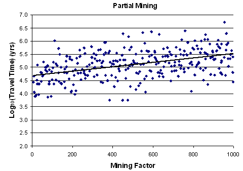
Figure TFIELD-79. Correlation Between the Random Mining Factor and log10 of Travel Time
Figure TFIELD-80. Head Contours and Particle Track for the Maximum-Travel-Time T Field (d03r01-R3) for the Partial-Mining Case. The WIPP LWB is the Red Box in the Center of the Figure and the Particle Track is the Blue Track Originating from the Approximate Center of the WIPP.
Figure TFIELD-81. Head Contours and Particle Track for the Minimum-Travel-Time T Field (d09r06-R2) for the Partial-Mining Case. The WIPP LWB is the Red Box in the Center of the Figure and the Particle Track is the Blue Track Originating from the Approximate Center of the WIPP.
Figure TFIELD-82. Head Contours and Particle Track for the Median-Travel-Time T Field (d13r07-R2) for the Partial-Mining Case. The WIPP LWB is the Red Box in the Center of the Figure and the Particle Track is the Blue Track Originating from the Approximate Center of the WIPP.
Figure TFIELD-83. Head Contours and Particle Track for the Maximum-Travel-Time T Field (d22r06-R2) for the Full-Mining Case. The WIPP LWB is the Red Box in the Center of the Figure and the Particle Track is the Blue Track Originating from the Approximate Center of the WIPP.
Figure TFIELD-84. Head Contours and Particle Track for the Minimum-Travel-Time T Field (d03r03-R3) for the Full-Mining Case. The WIPP LWB is the Red Box in the Center of the Figure and the Particle Track is the Blue Track Originating from the Approximate Center of the WIPP.
Figure TFIELD-85. Head Contours and Particle Track for the Median-Travel-Time T Field (d12r08-R3) for the Full-Mining Case. The WIPP LWB is the Red Box in the Center of the Figure and the Particle Track is the Blue Track Originating from the Approximate Center of the WIPP.
Observed Culebra transmissivity has been related to three deterministic factors: the thickness of overburden above the Culebra, the presence or absence of dissolution of the upper Salado, and the presence or absence of halite in units above and below the Culebra. Culebra transmissivity is also related to the occurrence of open, interconnected fractures, which cannot be mapped as easily as the other three factors and must be treated stochastically. A linear-regression model for Culebra transmissivity has been developed based on these factors that provides an excellent match to the observed data, and can be tested through the collection of additional data. This model was used to create 500 stochastic realizations of the distribution of Culebra transmissivity (“base” T fields) in the vicinity of the WIPP site.
A MODFLOW-2000 modeling domain was defined extending 30.7 km (19.1 mi) north-south and 22.4 km (13.9 mi) east-west, roughly centered on the WIPP site. This domain was discretized into 68,768 uniform 100-m (328-ft) by 100-m (328-ft) cells. Water-level measurements made in 37 wells in late 2000 were used to define “steady-state” head conditions and constant-head boundary conditions on the northern, eastern, and southern extremes of the model domain. No-flow boundaries down the arms of Nash Draw, representing flow lines, were used on the western side of the model domain, reducing the number of active cells to 53,769.
MODFLOW-2000 and PEST were used to calibrate 146 of the base T fields to steady-state heads and transient drawdown responses to seven large-scale pumping tests. This calibration was done by using 100 pilot points to adjust the transmissivity values within the model domain to improve the fit to the observed heads. The pilot points were used to adjust a residual T field that was combined with a previously created base T field to yield the final calibrated T field. Of the 146 T fields, 121 were judged to be adequately calibrated for use in WIPP compliance calculations by virtue of being from a single population with respect to the CDF of travel times from a point above the center of the WIPP disposal panels to the LWB. From these 121 T fields, the 100 having the best objective fit measures were selected for further use.
The EPA requires that the potential effects of future potash mining be taken into account when evaluating the performance of the WIPP disposal system. Accordingly, transmissivities in the areas within the model domain where current or future mining might affect the Culebra were scaled by a random multiplier between 1 and 1,000 obtained from LHS. A single multiplier was used for each T field, applied first to the areas outside the WIPP LWB that might be mined to create a partial-mining T field, and then to the areas both inside and outside the LWB that might be mined to create a full-mining T field. The LHS was performed three times to create three replicates of T fields, leading to a total of 600 T fields. The MODFLOW-2000 water “budget” files from forward runs of these 600 T fields provided the input to radionuclide-transport calculations using SECOTP2D.
In all cases (no mining, partial mining, and full mining), the particle tracks on the T fields show travel times that are longer than those calculated for the T fields used in the CCA. In the case of the T fields unaltered for the effects of mining, the longer travel times are caused by a shift of relatively high-T from the southeastern to the southwestern portion of the WIPP site relative to the CCA T fields. In the case of the T fields altered for full and partial mining, the longer travel times are the combined result of the westward shift of high-T discussed above and a change in the definition of the areas to be mined that resulted in less water entering the Culebra on the WIPP site.
Beauheim, R.L. 1987. Interpretations of Single-Well Hydraulic Tests Conducted at and near the Waste Isolation Pilot Plant (WIPP) Site, 1983–1987. SAND87-0039. Albuquerque, NM: Sandia National Laboratories...\..\references\Others\Beauheim_1987_Interpretations_of_Single_Well_Hydraulic_Tests_SAND87_0039.pdf
Beauheim, R.L. 2002a. Analysis Plan for Evaluation of the Effects of Head Changes on Calibration of Culebra Transmissivity Fields(Revision 1). AP-088. ERMS 524785. Carlsbad, NM: Sandia National Laboratories...\..\references\Others\Beauheim_2002_Analysis_Plan_for_the_Evaluation_of_the_Effects_of_Head_Changes_ERMS524785.pdf
Beauheim, R.L. 2002b. Routine Calculations Report in Support of Task 3 of AP-088: Calculation of Culebra Freshwater Heads in 1980, 1990, and 2000 for Use in T-Field Calibration. ERMS 522580. Carlsbad, NM: Sandia National Laboratories...\..\references\Others\Beauheim_2002_Routine_Calculations_Report_Support_of_Task_3_of_AP_088_ERMS522580.pdf
Beauheim, R.L. 2002c. Analysis Package for Interpretation of 1984 H-3 Pumping Tests. ERMS 523905. Carlsbad, NM: Sandia National Laboratories...\..\references\Others\Beauheim_2002_Analysis_Pckg_for_Interpretation_of_1984_H3_Pumping_Tests_ERMS523905.pdf
Beauheim, R.L. 2003. Analysis Report for AP-100, Task 1: Development and Application of Acceptance Criteria for Culebra Transmissivity (T) Fields. ERMS 531136. Carlsbad, NM: Sandia National Laboratories...\..\references\Others\Beauheim_2003_Analysis_Report_AP100_Task_1_Development_and_Application_of_Acceptance_Criteria_ERMS531136.pdf
Beauheim, R.L., and B.L. Fox. 2003. Records Package for AP-088, Task 4; Conditioning of Base T Fields to Transient Heads: Compilation and Reduction of Transient Head Data. ERMS 527572. Carlsbad, NM: Sandia National Laboratories...\..\references\Others\Beauheim_Fox_2003_Records_Package_for_AP_088_Task_4_ERMS527572.pdf
Beauheim, R.L., and R.M. Holt. 1990. “Hydrogeology of the WIPP Site.” Geological and Hydrological Studies of Evaporites in the Northern Delaware Basin for the Waste Isolation Pilot Plant (WIPP), New Mexico (pp. 131–79). Geological Society of America Field Trip No. 14 Guidebook. Dallas: Dallas Geological Society...\..\references\Others\Beauheim_Holt_1990_Hydrogeology_of_the_WIPP_Site.pdf
Beauheim, R.L., and G.J. Ruskauff. 1998. Analysis of Hydraulic Tests of the Culebra and Magenta Dolomites and Dewey Lake Redbeds Conducted at the Waste Isolation Pilot Plant Site. SAND98-0049. ERMS 251839. Albuquerque: Sandia National Laboratories...\..\references\Others\Beauheim_and_Ruskauff_1998_SAND98_0049_Analysis_of_Hydraulic_Tests.pdf
Corbet, T.F., and P.M. Knupp. 1996. The Role of Regional Groundwater Flow in the Hydrogeology of the Culebra Member of the Rustler Formation at the Waste Isolation Pilot Plant (WIPP), Southeastern New Mexico. SAND96-2133. ERMS 243482. Albuquerque: Sandia National Laboratories...\..\references\Others\Corbet_Knupp_1996_The_Role_of_Regional_Groundwater_Flow_SAND96_2133.pdf
Currie, J.B., and S.O. Nwachukwu. 1974. “Evidence on Incipient Fracture Porosity in Reservoir Rocks at Depth.” Bulletin of Canadian Petroleum Geology, vol. 22: 42–58...\..\references\Others\Currie_Nwachukwu_1974_Evidence_on_Fracture.pdf
Davies, P.B. 1989. Variable-Density Ground-Water Flow and Paleohydrology in the Waste Isolation Pilot Plant (WIPP) Region, Southeastern New Mexico. Open-File Report 88-490. ERMS 238854. Albuquerque: U.S. Geological Survey...\..\references\Others\Davies_1989_Variable_Density_Groundwater_Flow_Open_File_Report_88_490.pdf
Deutsch, C.V., and A.G. Journel. 1998. GSLIB: Geostatistical Software Library and User’s Guide. Version 2.0, 2nd ed. New York: Oxford UP...\..\references\Others\Deutsch_Journel_1998_GSLIB.pdf
Doherty, J. 2002. PEST: Model-Independent Parameter Estimation User Manual. 4th ed. Brisbane: Watermark Numerical Computing...\..\references\Others\Doherty_2004_Manual_for_PEST.pdf
Goovaerts, P. 1997. Geostatistics for Natural Resources Evaluation. New York: Oxford UP...\..\references\Others\Goovaerts_1997_Geostatistics.pdf
Harbaugh, A.W., E.R. Banta, M.C. Hill, and M.G. McDonald. 2000. MODFLOW-2000: The U.S. Geological Survey Modular Ground-Water Model—User Guide to Modularization Concepts and the Ground-Water Flow Process. Open File Report 00-92. Reston, VA: U.S. Geological Survey...\..\references\Others\Harbaugh_Banta_Hill_and_McDonald_2000_MODFLOW_2000_Open_File_Report_00_92.pdf
Holt, R.M. 1997. Conceptual Model for Transport Processes in the Culebra Dolomite Member, Rustler Formation. SAND97-0194. Albuquerque: Sandia National Laboratories...\..\references\Others\Holt_1997_Conceptual_Model_for_Transport_Processes_SAND97_0194.pdf
Holt, R.M., and D.W. Powers. 1988. Facies Variability and Post-Depositional Alteration within the Rustler Formation in the Vicinity of the Waste Isolation Pilot Plant, Southeastern New Mexico. DOE/WIPP 88-004. ERMS 242145. Carlsbad, NM: U.S. Department of Energy...\..\references\Others\Holt_Powers_1988_Facies_Variability_Post_Depositional_Alteration_Within_the_Rustler_Formation_88_004.pdf
Holt, R.M., and L. Yarbrough. 2002. Analysis Report: Task 2 of AP-088; Estimating Base Transmissivity Fields (July 8). ERMS 523889. Carlsbad, NM: Sandia National Laboratories...\..\references\Others\Holt_Yarbrough_2002_Analysis_Report_Task_2_of_AP_088_Estimating_Base_TFIELDs_ERMS523889.pdf
Holt, R.M., and L. Yarbrough. 2003a. Addendum to Analysis Report: Task 2 of AP-088: Estimating Base Transmissivity Fields. ERMS 527601. Carlsbad, NM: Sandia National Laboratories...\..\references\Others\Holt_Yarbrough_2003_Addendum_to_Analysis_Report_Task_2_of_AP_088_ERMS527601.pdf
Holt, R.M., and L. Yarbrough. 2003b. Addendum 2 to Analysis Report: Task 2 of AP-088; Estimating Base Transmissivity Fields (May 11). ERMS 529416. Carlsbad, NM: Sandia National Laboratories...\..\references\Others\Holt_Yarbrough_2003_Addendum_2_to_Analysis_Report_Task_2_of_AP_088_ERMS529416.pdf
Hunter, R.L. 1985. A Regional Water Balance for the Waste Isolation Pilot Plant (WIPP) Site and Surrounding Area. SAND84-2233. Albuquerque: Sandia National Laboratories...\..\references\Others\Hunter_1985_A_Regional_Water_Balance_for_WIPP_SAND84_2233.pdf
LaVenue, A.M. 1996. Analysis of the Generation of Transmissivity Fields for the Culebra Dolomite. ERMS 240517. Carlsbad, NM: Sandia National Laboratories...\..\references\Others\Lavenue_1996_Analysis_of_the_Generation_of_Transmissivity_Fields_for_Culebra_Dolomite_ERMS240517.pdf
LaVenue, A.M., and B.S. RamaRao. 1992. A Modeling Approach to Address Spatial Variability within the Culebra Dolomite Transmissivity Field. SAND92-7306. Albuquerque: Sandia National Laboratories...\..\references\Others\LaVenue_RamaRao_1992_A_Modeling_Approach_to_Address_Spatial_Variability_SAND92_7306.pdf
LaVenue, A.M., T.L. Cauffman, and J.F. Pickens. 1990. Ground-Water Flow Modeling of the Culebra Dolomite. Volume I: Model Calibration. SAND89-7068/1. Albuquerque: Sandia National Laboratories...\..\references\Others\LaVenue_Cauffman_Pickens_1990_Groundwater_Flow_Modeling_Vol1_SAND89_7068_1.pdf
Leigh, C., R. Beauheim, and J. Kanney. 2003. Analysis Plan for Calculations of Culebra Flow and Transport: Compliance Recertification Application. AP-100. ERMS 530172. Carlsbad, NM: Sandia National Laboratories...\..\references\Others\Leigh_Beauheim_Kanney_2003_AP_for_Calculations_of_Culebra_Flow_and_Transport_ERMS530172.pdf
Long, J. 2004. Execution of Performance Assessment for the Compliance Recertification Application (CRA1)(Revision 0). ERMS 530170. Carlsbad, NM: Sandia National Laboratories...\..\references\Others\Long_2004_Execution_of_PA_for_the_CRA_CRA1_Rev0_ERMS530170.pdf
Lowry, T.S. 2003. Analysis Report: Task 5 of AP-088; Evaluation of Mining Scenarios. ERMS 531138. Carlsbad, NM: Sandia National Laboratories...\..\references\Others\Lowry_2003_Analysis_Report_Task_5_of_AP088_Evaluation_of_Mining_Scenarios_ERMS531138.pdf
McKenna, S.A., and D.B. Hart. 2003a. Analysis Report: Task 3 of AP-088; Conditioning of Base T Fields to Steady-State Heads. ERMS 529633. Carlsbad, NM: Sandia National Laboratories...\..\references\Others\McKenna_Hart_2003_Analysis_Report_Task_3_AP088_ERMS529633.pdf
McKenna, S.A., and D.B. Hart. 2003b. Analysis Report: Task 4 of AP-088; Conditioning of Base T Fields to Transient Heads. ERMS 531124. Carlsbad, NM: Sandia National Laboratories...\..\references\Others\McKenna_Hart_2003_Analysis_Report_Task_4_AP088_ERMS531124.pdf
Meigs, L.C., and J.T. McCord. 1996. Physical Transport in the Culebra Dolomite (July 11). ERMS 237450. Carlsbad, NM: Sandia National Laboratories...\..\references\Others\Meigs_McCord_1996_Physical_Transport_in_Culebra_Dolmite_WPO37450.pdf
Mercer, J.W. 1983. Geohydrology of the Proposed Waste Isolation Pilot Plant Site, Los Medaños Area, Southeastern New Mexico. Water-Resources Investigations Report 83-4016. Albuquerque: U.S. Geological Survey...\..\references\Others\Mercer_1983_Geohydrology_of_Proposed_WIPP_83_4016.pdf
Pannatier, Y. 1996. VARIOWIN: Software for Spatial Data Analysis in 2D. New York: Springer...\..\references\Others\Pannatier_1996_VARIOWIN.pdf
Powers, D.W. 2002a. Analysis Report: Task 1 of AP-088; Construction of Geologic Contour Maps (April 17). ERMS 522086. Carlsbad, NM: Sandia National Laboratories...\..\references\Others\Powers_2002_Analysis_Report_Task_1_of_AP088_ERMS522086.pdf
Powers, D.W. 2002b. Addendum to Analysis Report: Task 1 of AP-088; Construction of Geologic Contour Maps. ERMS 523886. Carlsbad, NM: Sandia National Laboratories Center...\..\references\Others\Powers_2002_Addendum_to_Analysis_Report_Task_1_of_AP088_ERMS523886.pdf
Powers, D.W. 2003. Addendum 2 to Analysis Report: Task 1 of AP-088; Construction of Geologic Contour Maps. ERMS 525199. Carlsbad, NM: Sandia National Laboratories...\..\references\Others\Powers_2003_Addendum2_to_Analysis_Report_Task_1_of_AP088_ERMS525199.pdf
Powers, D.W., and R.M. Holt. 1990. “Sedimentology of the Rustler Formation near the Waste Isolation Pilot Plant (WIPP) Site.” Geological and Hydrological Studies of Evaporites in the Northern Delaware Basin for the Waste Isolation Pilot Plant (WIPP), New Mexico (pp. 79–106). Geological Society of America Field Trip No. 14 Guidebook. Dallas: Dallas Geological Society...\..\references\Others\Powers_Holt_1990_Sedimentology.pdf
Powers, D.W., and R.M. Holt. 1995. Regional Geologic Processes Affecting Rustler Hydrogeology. ERMS 244173. Carlsbad, NM: Sandia National Laboratories...\..\references\Others\Powers_Holt_1995_Regional_Geologic_Processes_Affecting_Rustler_Hydrogeology_ERMS244173.pdf
Powers, D.W., and R.M. Holt. 1999. “The Los Medaños Member of the Permian (Ochoan) Rustler Formation.” New Mexico Geology, vol. 21, no. 4: 97–103. ERMS 532368. ..\..\references\Others\Powers_Holt_1999_The_Los_Medanos_Member_of_the_Permian_Rustler_Formation.pdf
Powers, D.W., and R.M. Holt. 2000. “The Salt That Wasn’t There: Mudflat Facies Equivalents to Halite of the Permian Rustler Formation, Southeastern New Mexico.” Journal of Sedimentary Research, vol. 70: 29–36. ERMS 532369. ..\..\references\Others\Powers_and_Holt_2000_The_Salt_that_wasnt_there.pdf
Powers, D.W., R.M. Holt, R.L. Beauheim, and S.A. McKenna. 2003. “Geological Factors Related to the Transmissivity of the Culebra Dolomite Member, Permian Rustler Formation, Delaware Basin, Southeastern New Mexico.” Evaporite Karst and Engineering/Environmental Problems in the United States (pp. 211–18). Circular 109. Norman, OK: Oklahoma Geological Survey...\..\references\Others\Powers_Holt_Beauheim_McKenna_2003_Geological_Factors_Related_to_the_Transmissivity.pdf
Ramsey, J., M. Wallace, and H.N. Jow. 1996. Analysis Package for the Culebra Flow and Transport Calculations (Task 3) of the Performance Assessment Analyses Supporting the Compliance Certification Application (CCA). AP-019. ERMS 240516. Carlsbad, NM: Sandia National Laboratories...\..\references\Others\Ramsey_Wallace_Jow_1996_Analysis_Package_for_Culebra_Flow_and_Transport_Calculations_WPO40516.pdf
Roberts, R.M. 2002. nSIGHTS User Manual (Version 1.0). ERMS 522061. Carlsbad, NM: Sandia National Laboratories...\..\references\Others\Roberts_2002_nSIGHTS_User_Manual_Document_Version_1_ERMS522061.pdf
Rudeen, D.K. 2003. User’s Manual for DTRKMF Version 1.00. ERMS 523246. Carlsbad, NM: Sandia National Laboratories...\..\references\Others\Rudeen_2003_Users_Manual_for_DTRKMF_Version_1_ERMS523246.pdf
Snyder, R.P. 1985. Dissolution of Halite and Gypsum, and Hydration of Anhydrite to Gypsum, Rustler Formation, in the Vicinity of the Waste Isolation Pilot Plant, Southeastern New Mexico. Open-File Report 85-229. Denver: U.S. Geological Survey...\..\references\Others\Snyder_1985_Dissolution_of_Halite_and_Gypsum_and_Hydration_of_Anhydrite_to_Gypsum.pdf
U.S. Bureau of Land Management (BLM). 1993. Preliminary Map Showing Distribution of Potash Resources, Carlsbad Mining District, Eddy & Lea Counties, New Mexico. Roswell. WIPP Records Center, Carlsbad, NM, ERMS 525210...\..\references\Others\BLM_1993_Preliminary_Map_ERMS525210.pdf
U.S. Department of Energy (DOE). 1996. Title 40 CFR Part 191 Compliance Certification Application for the Waste Isolation Pilot Plant (October). 21 vols. DOE/CAO 1996-2184. Carlsbad, NM: Carlsbad Area Office...\..\references\CCA\CCA.htm
U.S. Department of Energy (DOE). 2004. Title 40 CFR Part 191 Compliance Recertification Application for the Waste Isolation Pilot Plant (March). 10 vols. DOE/WIPP 2004-3231. Carlsbad, NM: Carlsbad Field Office...\..\references\CRA-2004\CRA-2004.htm
U.S. Environmental Protection Agency (EPA). 1996. “40 CFR Part 194: Criteria for the Certification and Recertification of the Waste Isolation Pilot Plant’s Compliance with the 40 CFR Part 191 Disposal Regulations; Final Rule.” Federal Register, vol. 61 (February 9, 1996): 5223–45...\..\references\Others\EPA_61_FR_5224_5245_February_9_1996.pdf
U.S. Geological Survey (USGS). 2002. The National Map Seamless Server. <http://seamless.usgs.gov/website/seamless/viewer.htm>.http://seamless.usgs.gov/website/seamless/viewer.htm
Wallace, M. 1996. Records Package for Screening Effort NS11: Subsidence Associated with Mining Inside or Outside the Controlled Area (November 21). ERMS 412918. Carlsbad, NM: Sandia National Laboratories...\..\references\Others\Wallace_1996_Records_Package_for_Screening_Effort_NS11_ERMS412918.pdf
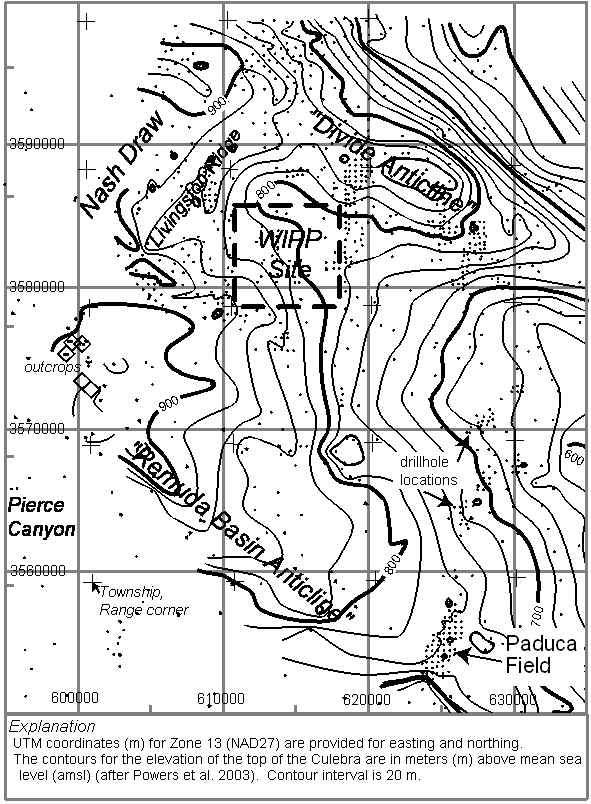
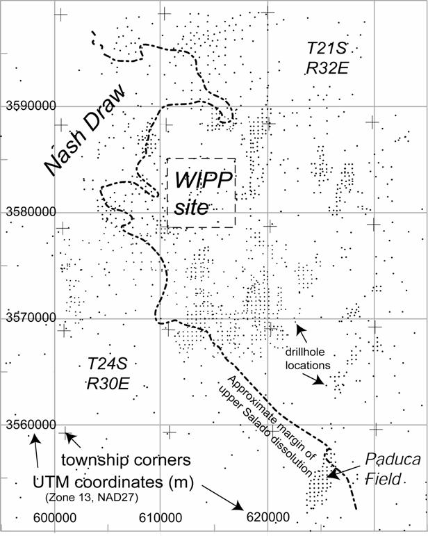

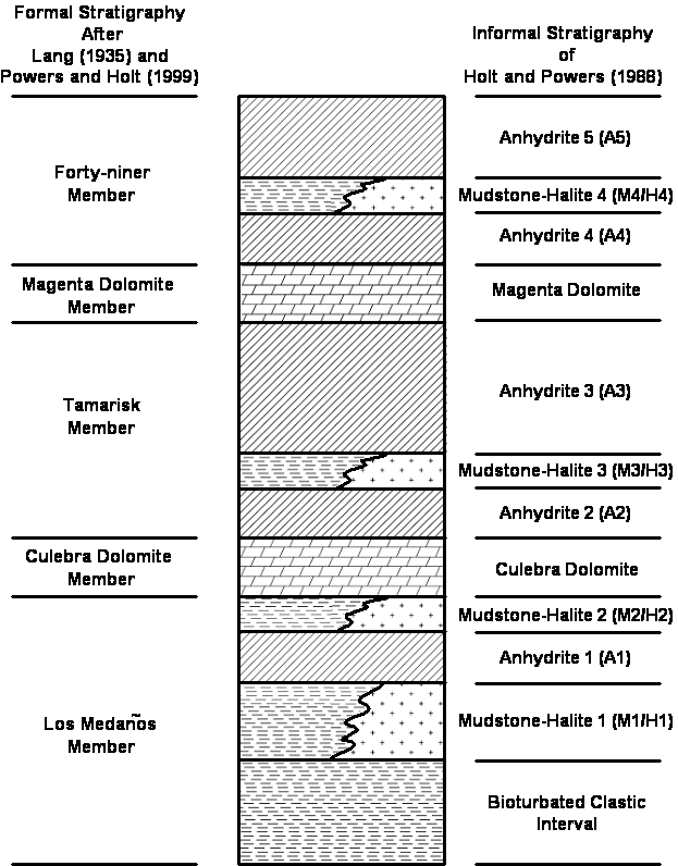
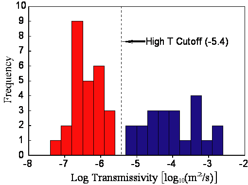
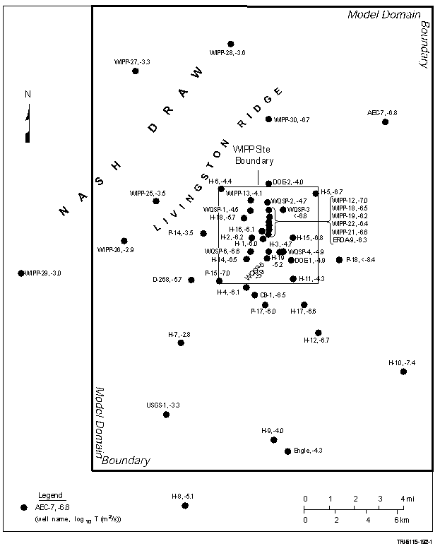
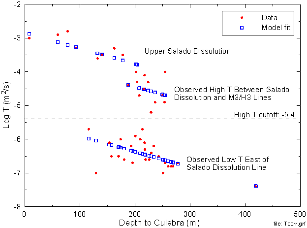
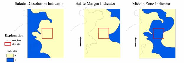
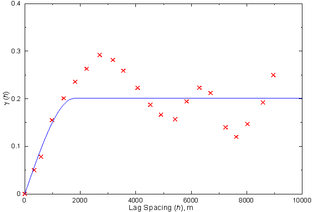
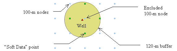
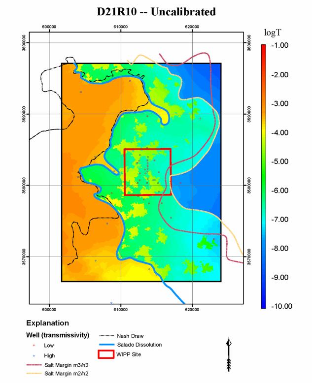
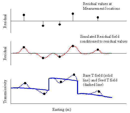
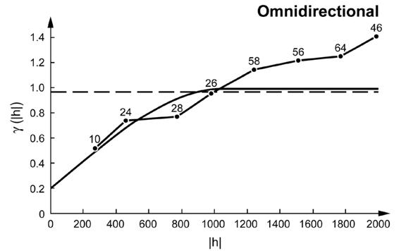
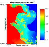
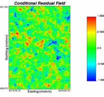
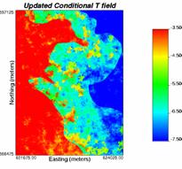
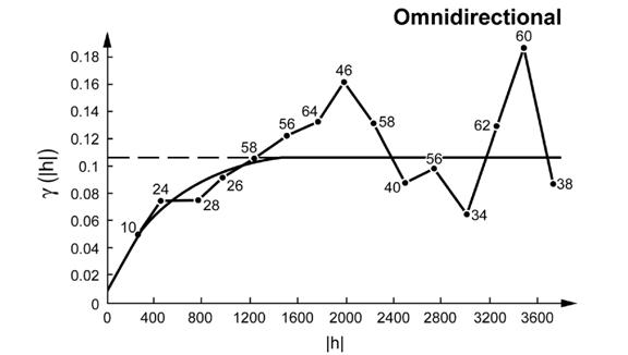
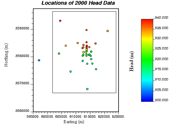
 (TFIELD.7)
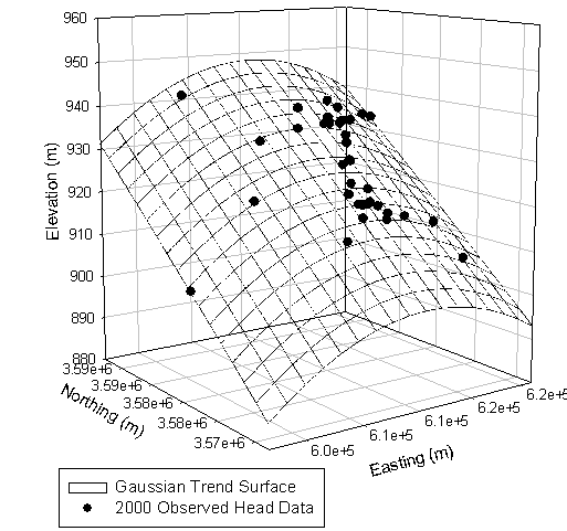
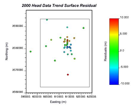

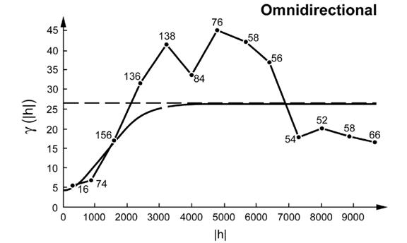
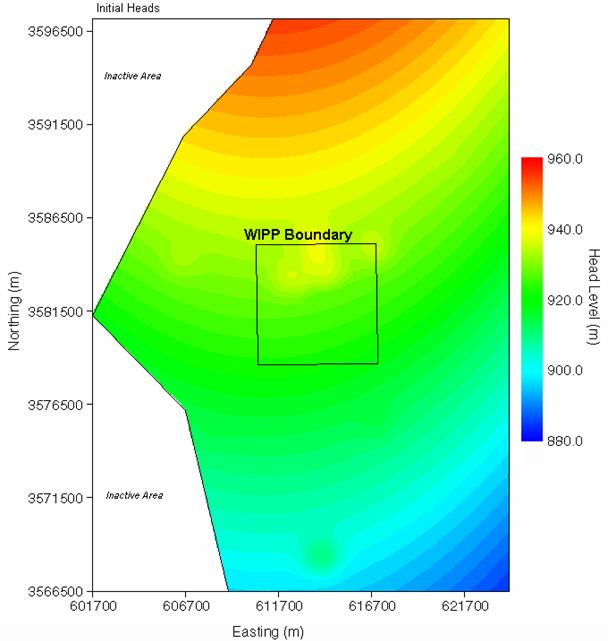

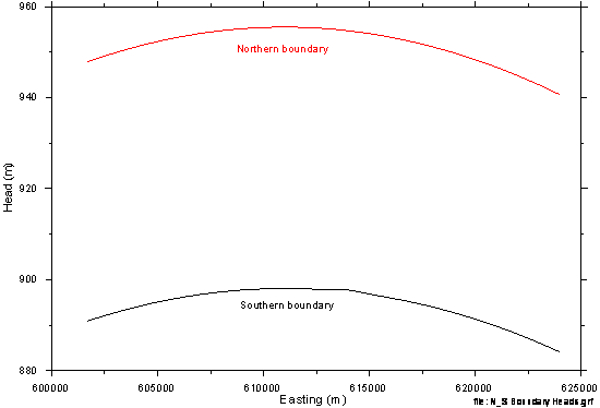
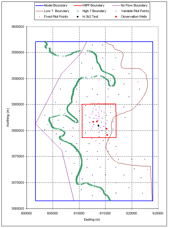
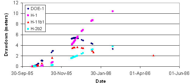
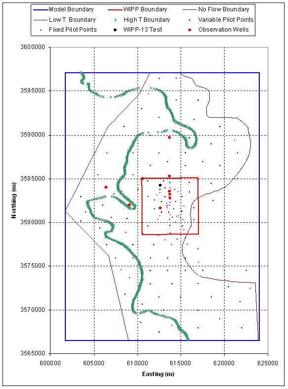

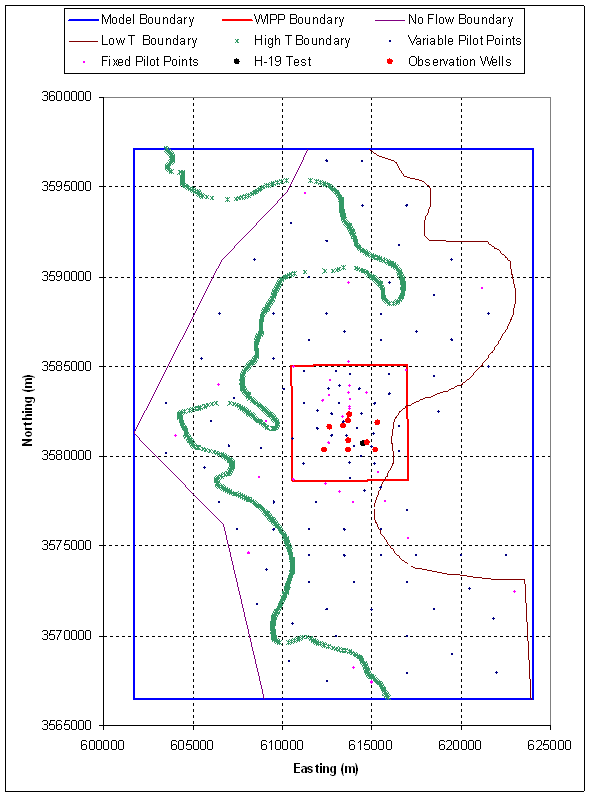
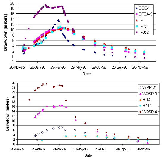
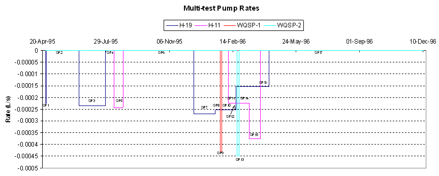
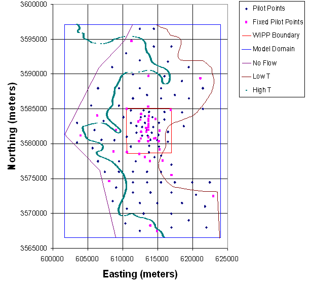
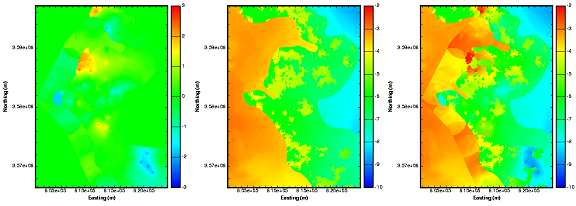
 (
(