PORSURF-1.0 Introduction

Both creep closure of the salt and the presence of either brine or gas in the U.S. Department of Energy (DOE) Waste Isolation Pilot Plant (WIPP) waste disposal region influence time-dependent changes in void volume in the waste disposal area. As a consequence, these processes influence two-phase fluid flow of brine and gases through the disposal area and its capacity for storing fluids. For performance assessment (PA), a porosity surface method is used to indirectly couple mechanical closure with two-phase fluid flow calculations implemented in the BRAGFLO code (see Appendix PA-2014, Section PA-4.2 ). The porosity surface approach is used because current codes are not capable of fully coupling creep closure, waste consolidation, brine availability, and gas production and migration. The porosity surface method incorporates the results of closure calculations obtained from the SANTOS code, a quasistatic, large deformation, finite element structural analysis code (Stone 1997a). The adequacy of the method is documented in Freeze (Freeze 1996), who concludes that the approximation is valid so long as the rate of room pressurization in final calculations is bounded by the room pressurization history used to develop the porosity surface.

The porosity surface used in the Compliance Recertification Application (CRA) of 2014 (CRA-2014) PA is the same surface used for the Compliance Certification Application (CCA) (U.S. DOE 1996), the CRA of 2004 (CRA-2004) (U.S. DOE 2004), and the CRA of 2009 (CRA-2009) (U.S. DOE 2009). Consequently, the models and parameters used to calculate this surface are unchanged from the CCA PA. For information on the porosity surface used in the CCA PA, see the CCA, Appendix PORSURF (U.S. DOE 1996).

A separate analysis considered the potential effects on repository performance of uncertainty in the porosity surface (U.S. DOE 2009, Appendix MASS-2009, Section MASS-21.0 ). Uncertainty in the porosity surface can arise from heterogeneity in the rigidity of waste packages and from uncertain spatial arrangements of waste in the repository. The analysis considered four porosity surfaces, including the surface from the CCA, which represented various bounding combinations of waste package rigidity and waste initial porosity. The analysis concluded that uncertainty in the porosity surface did not have significant effects on repository performance, and recommended the continued use of the CCA porosity surface in PA.

PORSURF-2.0 Creep Closure Method

Creep closure is accounted for in BRAGFLO by changing the porosity of the waste disposal area according to a table of porosity values, termed the porosity surface. The porosity surface is generated using SANTOS, a nonlinear finite element code. Disposal room porosity is calculated over time, for different rates of gas generation and gas production potential, to construct a three-dimensional porosity surface representing changes in porosity as a function of pressure and time over the 10,000-year simulation period.

The completed porosity surface is compiled in tabular form and is used in the solution of the gas and brine mass balance equations presented in Appendix PA-2014, Section PA-4.2.1. Porosity is interpolated from the porosity surface corresponding to the calculated gas pressure at time step t_n . This is done iteratively, as decreases in the porosity will increase the pressure. The closure data provided by SANTOS can be viewed as a series of surfaces, with any gas generation history computed by BRAGFLO constrained to fall on this surface. Various techniques described in Freeze, Larson, and Davies (Freeze, Larson, and Davies 1995) were used to check the validity of this approach, and it was found to be a reasonable representation of the behavior observed in the complex models.

In SANTOS, the gas pressure in the disposal room at time t_n is computed from the ideal gas law by the following relationship:

where N is the number of moles of gas at time t_n , R is the universal gas constant (8.31 m³∙Pa/mol∙K), T is the absolute temperature in kelvins (K) (constant at 300 K), and V is the free volume of the room at time t_n . The number of moles of gas is computed as

where is the gas generation rate (mol/drum/yr) at time t for the scaling factor f and N_drums is the number of drums of waste in the room (6804 drums/room). The base gas generation rate in SANTOS is

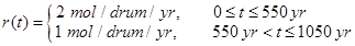
The base gas generation rate is representative of relatively high gas production rates from both microbial degradation of cellulosic, plastic, and rubber materials and from anoxic corrosion of iron-based metals (Appendix PA-2014, Section PA-4.2.5 ; Butcher 1997a; Roselle 2013). To provide a range of SANTOS results that spans the possible range of pressure computed by BRAGFLO, the gas generation rate is varied by the scaling factor f. Thirteen values of f are used to construct the porosity surface: f = 0.0, 0.025, 0.05, 0.1, 0.2, 0.4, 0.5, 0.6, 0.8, 1.0, 1.2, 1.6, and 2.0. The condition f = 0 represents the state of the repository when no gas is produced; f = 2 represents twice the base gas generation rate.

In SANTOS, gas generation is included to introduce a range of values for gas pressure during room closure, thereby capturing its effects. The use of the scaling factor f ensures that SANTOS results span a wide range of possible gas generation rates and potentials.

PORSURF-3.0 Conceptual Model for Porosity Surface

The ability of salt to deform with time, eliminate voids, and create an impermeable barrier around the waste was one of the principal reasons for locating the WIPP repository in a bedded salt formation (National Academy of Sciences National Research Council 1957, pp. 4,5). The creep closure process is a complex and interdependent series of events starting after a region within the repository is excavated. Immediately upon excavation, the equilibrium state of the rock surrounding the repository is disturbed, and the rock begins to deform and return to equilibrium. At equilibrium, deformation eventually ceases as the waste region has undergone as much compaction as is possible under the prevailing lithostatic stress field and the differential stresses in the salt approach zero.

Creep closure of a room begins immediately upon excavation and causes the volume of the cavity to decrease. If the room were empty, rather than partially filled with waste, closure would proceed until the void volume created by the excavation is eliminated; the surrounding halite would then return to its undisturbed, uniform stress state. In a waste-filled room, the rock will contact the waste and the rate of closure will decrease as the waste compacts and stiffens. Closure will eventually cease when the waste can take the full overburden load without further deformation. Initially, unconsolidated waste can support only small loads, but as the room continues to close after contact with the waste, the waste will consolidate and support a greater portion of the overburden load.

The presence of gas in the room will retard the closure process due to pressure buildup. As the waste consolidates, pore volume is reduced and pore pressure increases (using the ideal gas law). In this process, the waste can be considered to be a skeleton structure immersed in a pore fluid (the gas). As the pore pressure increases, less overburden weight is carried by the skeleton, and more support is provided by the gas. If the gas pressure increases to lithostatic pressure, the pore pressure alone is sufficient to support the overburden.

PORSURF-4.0 SANTOS Numerical Analyses

Computing repository creep closure is a particularly challenging structural engineering problem because the rock surrounding the repository continually deforms with time until equilibrium is reached. Not only is the deformation of the salt inelastic, but it also involves large deformations that are not customarily addressed with conventional structural deformation codes. In addition, the formation surrounding the repository is heterogeneous in composition, containing various parting planes and interbeds with different properties than the salt.

Waste deformation is also nonlinear, with large strains, and the response of a waste-filled room is complicated by the presence of gas. These complex characteristics of the materials making up the repository and its surroundings require the use of highly specialized constitutive models. Appropriate models have been built into the SANTOS code over a number of years. Principal components of these models include the following:

1. Disposal Room Configuration and Idealized Stratigraphy. Disposal room dimensions, computational configuration, and idealized stratigraphy are defined in the CCA, Appendix PORSURF, Attachment 1. The idealized stratigraphy is reproduced in Figure PORSURF-1.

2. Discretized Finite Element Model. A two-dimensional plane strain model, shown in Figure PORSURF-2, is used for the SANTOS analyses. The discretized model represents the room as one of an infinite number of rooms located at the repository horizon. The model contains 1,680 quadrilateral uniform-strain elements and 1,805 nodal points. Contact surfaces between the emplaced waste and the surfaces of the room are addressed. The justification for this model and additional detail on initial and boundary conditions are provided in the CCA, Appendix PORSURF, Attachment 1.

3. Geomechanical Models. Mechanical material response models and their corresponding property values are assigned to each region of the configuration. These models include:

A. A combined transient-secondary creep constitutive model for clean and argillaceous halite

B. An inelastic constitutive model for anhydrite

C. A volumetric plasticity model for the emplaced waste

D. Material properties are provided in the CCA, Appendix PORSURF, Attachment 1.

Continual testing and reviews of computer codes by the DOE and the U.S. Environmental Protection Agency (EPA) from before the CCA have shown that the use of SANTOS and its models are adequate for WIPP porosity surface calculations (e.g., Argüello and Holland 1996; WIPP PA 2003; U.S. EPA 2005).

The results of the SANTOS calculations are illustrated in Figure PORSURF-3 and Figure PORSURF-4. Figure PORSURF-3 shows disposal room porosity as a function of time for various values of the gas generation scaling factor f. Figure PORSURF-4 shows disposal room pressure as a function of time for various values of f. When f = 0, no gas is present in the disposal room; thus, disposal room pressure is zero for all times. This pressure curve is omitted from Figure PORSURF-4.

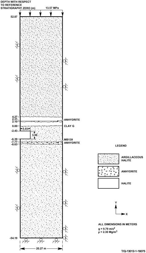
Figure PORSURF- 1. Stratigraphy Used for the Porosity Surface Calculations

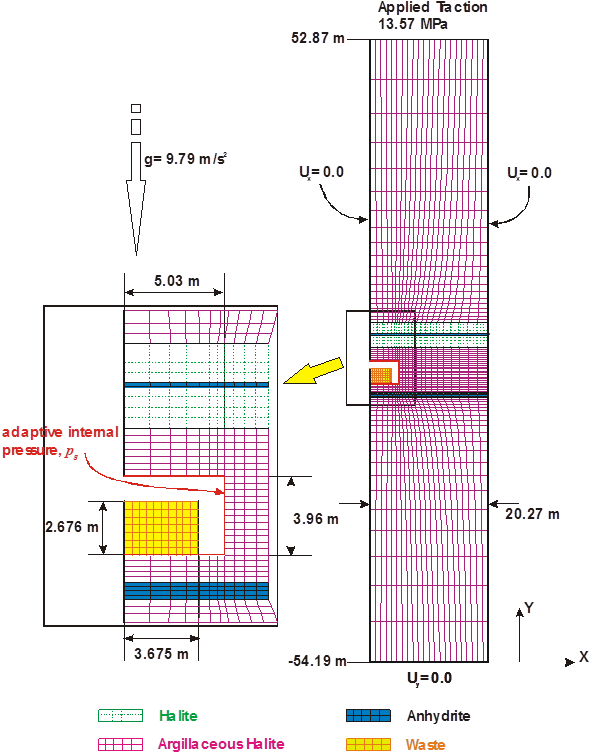
Figure PORSURF- 2. Mesh Discretization and Boundary Conditions Used for the Porosity Surface Calculations

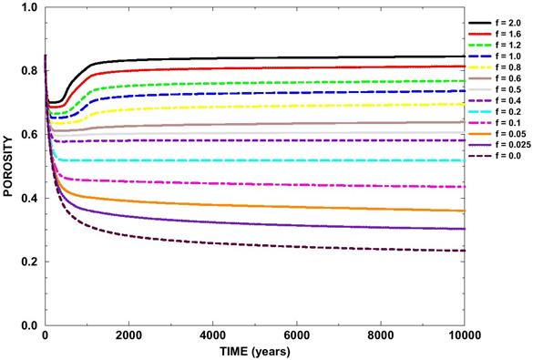
Figure PORSURF- 3. Disposal Room Porosity for Various Values of the Scaling Factor f

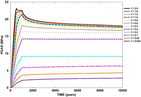
Figure PORSURF- 4. Disposal Room Pressure for Various Values of the Scaling Factor f

PORSURF-5.0 Implementation of Porosity Surface in BRAGFLO

As outlined above, the SANTOS program is used to calculate time-dependent porosities and pressures in the repository for a range of gas generation rates determined by the scaling factor f. Calculation with each value of f results in the porosity and pressure curves in Figure PORSURF-3 and Figure PORSURF-4.

The porosity calculated by SANTOS is the intrinsic, or true, porosity, which is defined as the ratio of the void volume to the current volume of a (deformable) element of waste. In contrast, porosity in BRAGFLO is defined as the ratio of void volume to the original volume of an element of waste. Mathematically, the BRAGFLO porosity, f _B , and the intrinsic porosity in SANTOS, f , are defined as

where V_void is the current void volume, V₀ is the original (total) volume, and V is the current (total) volume of a waste element.

The porosities shown in Figure PORSURF-3 are the porosities calculated by SANTOS to be used in BRAGFLO. The BRAGFLO porosities are related to the porosities calculated by SANTOS by correcting for deformation of the waste during repository closure. The relationship between f _B and f is given by

where f ₀ is the initial porosity of the waste. Note that the values of f _B and f are equal at the initial porosity before the waste starts to compact.

Brine pressures p_b (t) obtained in the waste disposal regions are used in conjunction with the results in Figure PORSURF-3 and Figure PORSURF-4 to estimate porosity in the waste-filled regions for the BRAGFLO calculations. In the CRA-2014 PA, brine pressure and gas pressure are set as equal in the waste-filled regions, i.e., capillary pressure is not included (see Appendix PA-2014, Section PA-4.2 ). This is unchanged from the CCA and previous two CRA PAs.

Given a value for p(t), BRAGFLO looks at the porosity surface to find indices for times in the porosity table so that

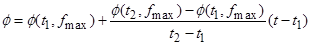
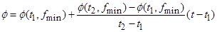
Next, BRAGFLO determines whether the current pressure is above the pressure curve in the interpolation table corresponding to the maximum f value or corresponding to the minimum f value in the table. If p lies above the curve formed by the points and , the porosity is calculated by interpolation using the following formula:

Similarly, if p lies below the curve formed by the points and , the porosity is calculated by interpolation using the following formula:

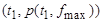
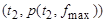
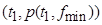
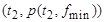
For values of p that do not lie above or below the maximum and minimum p(t, f ) curves in the interpolation table, BRAGFLO finds f values f ₁ and f ₂ so that the point (t, p) lies between two curves (t, p(t, f ₁)) and (t, p(t, f ₂)). This is illustrated in Figure PORSURF-5.

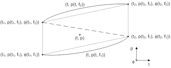
Figure PORSURF- 5. Location of Points in Porosity Table around Point (t, p)

Interpolation is performed on the triangle formed by the set of points that encloses the point (t, p). For example, in Figure PORSURF-5, the points constituting the lower triangle would be used for interpolation. Interpolation on the triangle is calculated from the areas of the three triangles in the plane of t and p that can be formed from the point (t, p) and the vertices of the enclosing triangle, as illustrated in Figure PORSURF-6. The porosity is then calculated from

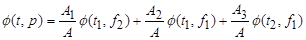
where A is the total area of the triangles in Figure PORSURF-6.

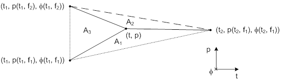
Figure PORSURF- 6. Triangular Interpolation to Determine the Porosity at (t, p)

At t = 0 (i.e., immediately after the operational period; see Appendix PA-2014, Section PA-4.2 ), interpolation is performed using the points and . This is because at t = 0, the two points vertically separated in Figure PORSURF-6 at are equal (the porosity is equal to the initial value at t = 0 for all values of f ).

PORSURF-6.0 Dynamic Closure of the North End and Hallways

The porosity surface method is not used to model the north end of the repository occupied by the experimental and operational regions. During development of the CCA PA, a supporting analysis compared brine and gas flow results for two models for closure of the north end of the repository: a dynamic closure model and a baseline model, in which the porosity and permeability of these regions were held constant (Vaughn, Lord, and MacKinnon 1995). The study examined the effect of these two approaches on brine releases to the accessible environment for both disturbed and undisturbed conditions, as well as the effects on brine pressures and brine saturations in the modeled regions. The study concluded that the baseline case (assuming constant low porosity and high permeability) consistently led to either similar or more conservative brine pressures and brine saturations, thereby overestimating potential releases relative to the dynamic consolidation case. Consequently, PA uses the simplifying case of constant porosity and permeability in the north end of the repository, rather than modeling dynamic closure of these areas.

PORSURF-7.0 Additional Information

The following attachments were included in the CCA, Appendix PORSURF (U.S. DOE 1996) to document additional details of the porosity surface method:

1. The CCA, Appendix PORSURF, Attachment 1, Proposed Model for the Final Porosity Surface Calculations. This memo documents preliminary configuration and constitutive property values for the final porosity surface calculations. Tables in the memo include elastic and creep properties for clean halite and argillaceous halite, volumetric strain data and material constants used in the volumetric-plasticity model for waste, and elastic and Drucker-Prager constants assigned to anhydrite Marker Bed 139. This attachment was supplemented and updated subsequent to the CCA by Butcher (Butcher 1997a and Butcher 1997b).

2. The CCA, Appendix PORSURF, Attachment 2, Baseline Inventory Assumptions for the Final Porosity Surface Calculations. This memo discusses the effect of changes in the Transuranic Waste Baseline Inventory Report on the SANTOS analyses.

3. The CCA, Appendix PORSURF, Attachment 3, Corrosion and Microbial Gas Generation Potentials. This memo discusses the rationale for the base gas production potentials of 1,050 mol per drum for corrosion and 550 mol per drum for microbial decay in the SANTOS analyses.

4. The CCA, Appendix PORSURF, Attachment 4, Resolution of Remaining Issues for the Final Disposal Room Calculations. This memo provides additional detail on the disposal room elevation, determination of plastic constants for transuranic waste, and determination of SANTOS input constants for clean halite, argillaceous halite, and anhydrite.

5. The CCA, Appendix PORSURF, Attachment 5, Sample SANTOS Input File for Disposal Room Analysis. A representative sample input file is provided in this attachment. This listing does not include the adaptive pressure boundary condition subroutine used to calculate the gas pressure in a disposal room (Stone 1997b).

6. The CCA, Appendix PORSURF, Attachment 6, Final Porosity Surface Data. This attachment provides SANTOS results for selected gas generation scaling factors f = 0.5, 1.0, and 2.0. This attachment was updated and published as a formal SAND report (Stone 1997b) subsequent to submittal of the CCA.

7. The CCA, Appendix PORSURF, Attachment 7, SANTOS - A Two-Dimensional Finite Element Program for the Quasistatic, Large Deformation, Inelastic Response of Solids. This report documents the SANTOS code.

PORSURF-8.0 References

(*Indicates a reference that has not been previously submitted.)

Argüello, J.G. and J.F. Holland. 1996. SANTOS - Verification and Qualification Document. ERMS 235675. Albuquerque, NM: Sandia National Laboratories. [PDF / Author]

Butcher, B.M. 1997a. A Summary of the Sources of Input Parameter Values for the Waste Isolation Pilot Plant Final Porosity Surface Calculations. SAND97-0796. Albuquerque, NM: Sandia National Laboratories. [PDF / Author]

Butcher, B.M. 1997b. Waste Isolation Pilot Plant Disposal Room Model. SAND97-0794. Albuquerque, NM: Sandia National Laboratories. [PDF / Author]

Freeze, G.A. 1996. Repository Closure-Reasoned Argument for FEP Issue DR12. ERMS 413328. Albuquerque, NM: Sandia National Laboratories. [PDF / Author]

Freeze, G.A., K.W. Larson, and P.B. Davies. 1995. Coupled Multiphase Flow and Closure Analysis of Repository Response to Waste-Generated Gas at the Waste Isolation Pilot Plant (WIPP). SAND93-1986. Albuquerque, NM: Sandia National Laboratories. [PDF / Author]

National Academy of Sciences-National Research Council (NAS-NRC). 1957. The Disposal of Radioactive Waste on Land. Publication 519. Washington, DC: National Academy of Sciences. [Author]

Roselle, G.T. 2013. Determination of Corrosion Rates from Iron/Lead Corrosion Experiments to be used for Gas Generation Calculations, Rev. 1. ERMS 559077. Carlsbad, NM: Sandia National Laboratories.* [PDF / Author]

Stone, C.M. 1997a. SANTOS - A Two-Dimensional Finite-Element Program for the Quasistatic, Large Deformation, Inelastic Response of Solids. SAND90-0543. Albuquerque, NM: Sandia National Laboratories. [PDF / Author]

Stone, C.M. 1997b. Final Disposal Room Structural Response Calculations. SAND97-0795. Albuquerque, NM: Sandia National Laboratories. [PDF / Author]

U.S. Department of Energy. (DOE) 1996. Title 40 CFR Part 191 Compliance Certification Application for the Waste Isolation Pilot Plant. 21 vols. DOE/CAO 1996-2184. Carlsbad, NM: Carlsbad Area Office. [Author]

U.S. Department of Energy. (DOE) 2004. Title 40 CFR Part 191 Compliance Recertification Application for the Waste Isolation Pilot Plant. 10 vols. DOE/WIPP 2004-3231. Carlsbad, NM: Carlsbad Field Office. [Author]

U.S. Department of Energy. (DOE) 2009. Title 40 CFR Part 191 Compliance Recertification Application for the Waste Isolation Pilot Plant. DOE/WIPP 09-3424. Carlsbad, NM: Carlsbad Field Office. [Author]

U.S. Environmental Protection Agency. (EPA) 2005. Technical Support Document for Section 194.27: SANTOS Computer Code in WIPP Performance Assessment. Docket No.: A-98-49, II-B1-17. Washington, DC: U.S. EPA Office of Radiation and Indoor Air. [PDF / Author]

Vaughn, P., M. Lord, and R. MacKinnon. 1995. DR-3: Dynamic Closure of the North-End and Hallways. Summary Memorandum of Record to D.R. Anderson; Subject: FEP Screening Issue DR-3; dated December 21, 1995. ERMS 230794. Albuquerque, NM: Sandia National Laboratories. [PDF / Author]

WIPP PA. 2003. Verification and Validation Plan/Validation Document for SANTOS (Version 2.1.7). ERMS 530091. Carlsbad, NM: Sandia National Laboratories. [PDF / Author]

Table of Contents

List of Figures

Acronyms and Abbreviations