PA-1.0 Introduction

This appendix presents the mathematical models used to evaluate performance of the Waste Isolation Pilot Plant (WIPP) disposal system and the results of these models for the 2014 Compliance Recertification Application (CRA-2014) Performance Assessment (PA). The term PA signifies an analysis that (1) identifies the processes and events that might affect the disposal system; (2) examines the effects of these processes and events on the performance of the disposal system; and (3) estimates the cumulative releases of radionuclides, considering the associated uncertainties, caused by all significant processes and events (section 191.12 [U.S. EPA 1993]). PA is designed to address three primary questions about the WIPP:

Q1: What processes and events that might affect the disposal system could take place at the WIPP site over the next 10,000 years?

Q2: How likely are the various processes and events that might affect the disposal system to take place at the WIPP site over the next 10,000 years?

Q3: What are the consequences of the various processes and events that might affect the disposal system that could take place at the WIPP site over the next 10,000 years?

In addition, accounting for uncertainty in the parameters of the PA models leads to a further question:

Q4: How much confidence should be placed in answers to the first three questions?

These questions give rise to a methodology for quantifying the probability distribution of possible radionuclide releases from the WIPP repository over the next 10,000 years and characterizing the uncertainty in that distribution due to imperfect knowledge about the parameters contained in the models used to predict releases. The containment requirements of section 191.13 require this probabilistic methodology.

This appendix is organized as follows: Section PA-1.1 summarizes changes made to the WIPP PA since the CRA-2009 PA (Clayton et al. 2008). Section PA-2.0 gives an overview and describes the overall conceptual structure of the CRA-2014 PA. The WIPP PA is designed to address the requirements of section 191.13, and thus involves three basic entities: (1) models for both the physical processes that take place at the WIPP site and the estimation of potential radionuclide releases that may be associated with these processes, (2) a probabilistic characterization of the uncertainty in the models and parameters that underlay the WIPP PA (to account for epistemic uncertainty), and (3) a probabilistic characterization of different futures that could occur at the WIPP site over the next 10,000 years (to account for aleatory uncertainty). Section PA-1.1 is supplemented by Appendix SCR-2014, which documents the results of the screening process for features, events, and processes (FEPs) that are retained in the conceptual models of repository performance, including those FEPs which have been modified since CRA-2009.

Section PA-3.0 describes the probabilistic characterization of different futures and summarizes the stochastic variables that represent future drilling and mining events in the PA. This characterization plays an important role in the construction of the complementary cumulative distribution function (CCDF) specified in section 191.13. Regulatory guidance and extensive review of the WIPP site identified exploratory drilling for natural resources and the mining of potash as the only significant disruptions at the WIPP site with the potential to affect radionuclide releases to the accessible environment.

Section PA-4.0 presents the mathematical models for both the physical processes that take place at the WIPP and the estimation of potential radionuclide releases. The mathematical models implement the conceptual models as prescribed in section 194.23, and permit the construction of the CCDF specified in section 191.13. Models presented in Section PA-4.0 include two-phase (i.e., gas and brine) flow in the vicinity of the repository; radionuclide transport in the Salado Formation (hereafter referred to as the Salado); releases to the surface at the time of a drilling intrusion due to cuttings, cavings, spallings, and direct brine releases (DBRs); brine flow in the Culebra Dolomite Member of the Rustler Formation (hereafter referred to as the Culebra); and radionuclide transport in the Culebra. Section PA-4.0 is supplemented by Appendices MASS-2014, TFIELD-2014, and PORSURF-2014. Appendix MASS-2014 discusses the modeling assumptions used in the WIPP PA. Appendix TFIELD-2014 discusses the generation of the transmissivity fields (T-fields) used to model groundwater flow in the Culebra. Appendix PORSURF-2014 presents results from modeling the effects of excavated region closure, waste consolidation, and gas generation in the repository.

Section PA-5.0 discusses the probabilistic characterization of parameter uncertainty, and summarizes the uncertain variables incorporated into the CRA-2014 PA, the distributions assigned to these variables, and the correlations between variables. Section PA-5.0 is supplemented by Kicker and Herrick (Kicker and Herrick 2013) and Appendix SOTERM-2014. Kicker and Herrick (Kicker and Herrick 2013) catalogs the full set of parameters used in the CRA-2014 PA. Appendix SOTERM-2014 describes the actinide source term for the WIPP performance calculations, including the mobile concentrations of actinides that may be released from the repository in brine.

Section PA-6.0 summarizes the computational procedures used in the CRA-2014 PA, including sampling techniques, sample size, statistical confidence for mean CCDF, generation of sample, generation of individual futures, construction of CCDFs, calculations performed with the models discussed in Section PA-4.0, construction of releases for each future, and the sensitivity analysis techniques in use.

Section PA-7.0 presents the results of the PA for an undisturbed repository. Releases from the undisturbed repository are determined by radionuclide transport in brine flowing from the repository to the Land Withdrawal Boundary (LWB) through the marker beds (MBs) or shafts. Releases in the undisturbed scenario are used to demonstrate compliance with the individual and groundwater protection requirements in 40 CFR Part 191 (section 194.51 and section 194.52).

Section PA-8.0 presents PA results for a disturbed repository. As discussed in Section PA-2.3.1, the only future events and processes in the analysis of disturbed repository performance are those associated with mining and deep drilling. Release mechanisms include direct releases at the time of the intrusion via cuttings, cavings, spallings, and DBR, and long-term releases via radionuclide transport up abandoned boreholes to the Culebra and thence to the LWB.

Section PA-9.0 presents the set of CCDFs resulting from the CRA-2014 PA. This material supports Section 194.34 of CRA-2014, which demonstrates compliance with the containment requirements of section 191.13. Section PA-9.0 presents the most significant output variables from the PA models, accompanied by sensitivity analyses to determine which subjectively uncertain parameters are most influential in the uncertainty of PA results.

The results of the PA for CRA-2014, as documented in Section PA-7.0, Section PA-8.0, and Section PA-9.0, confirm that direct releases from drilling intrusions are the major contributors to radionuclide releases to the accessible environment. In addition, the CRA-2014 PA results demonstrate that the WIPP continues to comply with the quantitative containment requirements in section 191.13(a).

The overall structure of Appendix PA-2014 is identical with that of the Appendix PA-2009 (U.S. DOE 2009). This appendix follows the approach used by Helton et al. (1998) to document the mathematical models used in the Compliance Certification Application (CCA) PA and the results of that analysis. Much of the content of this appendix derives from Helton et al. (1998); these authors' contributions are gratefully acknowledged.

PA-1.1 Changes since the CRA-2009 PA

As part of its review of the CRA-2009 (U.S. DOE 2009), the U.S. Environmental Protection Agency (EPA) requested changes to the CRA-2009 PA (Cotsworth 2009) including updates to the repository waste inventory, actinide solubilities, Culebra transmissivity fields, drilling parameters, and matrix partition coefficients. These changes were incorporated into the CRA-2009 Performance Assessment Baseline Calculation (CRA-2009 PABC) (Clayton et al. 2010). Repository performance with these requested changes was subsequently assessed by the EPA, and the WIPP was recertified in 2010 (U.S. EPA 2010a). The CRA-2009 PABC is the current regulatory baseline for the WIPP. The U.S. Department of Energy (DOE) continues to use the same PA methodology as in the CCA and the CRA-2009 PABC because changes that have been made since the EPA first certified the WIPP in 1998 do not impact PA methodology. A detailed presentation for the CCA PA methodology is provided in (Helton et al. (1998), Section 2).

In addition to including applicable changes from CRA-2009 incorporated in the CRA-2009 PABC, the CRA-2014 PA is updated based on new information since the CRA-2009 PABC. Information on the implementation of these updates is contained in Camphouse et al. (Camphouse et al.2013). Changes included in the CRA-2014 PA relative to the CRA-2009 PA are summarized in Table PA-1. Culebra transmissivity fields and matrix partition coefficients were updated as part of the CRA-2009 PABC; these updates are carried forward to the CRA-2014 PA. Updates to Culebra transmissivity fields (T-fields) and matrix partition coefficients are included in Table PA-1 for the sake of completeness as they are changes made since the CRA-2009 PA. Other changes between the CRA-2009 PA and the CRA-2009 PABC have been superseded by new information since the CRA-2009 PABC. The random seeds used in the CRA-2009 PABC are also used in the CRA-2014 PA. Use of the CRA-2009 PABC random seeds (and parameter ordering as applicable) results in identical sampled values for sampled parameters that are common to the CRA-2009 PABC and the CRA-2014 PA.

This section ends with motivations for and brief descriptions of each of the updates developed for and included in the CRA-2014 PA.

Table PA- 1. Changes since the CRA-2009 PA Incorporated in the CRA-2014 PA

WIPP Project Change	Summary of Change and Cross-Reference
Culebra Transmissivity Fields (Carried over from CRA-2009 PABC)	Culebra transmissivity fields are updated based on revised hydrogeologic factors for the Culebra (Appendix HYDRO-2014, Attachment TFIELD-2014).
Updated Culebra Matrix Partition Coefficients (Carried over from CRA-2009 PABC)	Updated to account for higher organic ligand concentrations in the WIPP waste inventory (Clayton 2009).
Panel Closure Design	The Option D panel closure system (PCS) design is replaced with the run-of-mine panel closure system (ROMPCS) design (see Sections PA-1.1.1 and PA-4.2.8).
Added Volume in the Repository Experimental Region	A volume of 60,335 cubic meters (m³) is added to the volume of the WIPP experimental region for Salt Disposal Investigation experiments (see Section PA-1.1.2).
Probability of Encountering Pressurized Brine during a Drilling Intrusion	A revised distribution is used for WIPP PA parameter GLOBAL:PBRINE (see Section PA-1.1.3).
Refinement to Steel Corrosion Rate	A revised distribution is used for WIPP PA parameter STEEL:CORRMCO2 (see Section PA-1.1.4).
Updated Waste Shear Strength	A revised distribution is used for WIPP PA parameter BOREHOLE:TAUFAIL (see Section PA-1.1.5).
Updated Waste Inventory Information	Inventory parameters in the CRA-2014 PA are updated to reflect information collected through December 31, 2011 (see Section PA-1.1.6).
Drilling Rate	The drilling rate increased from 59.8 to 67.3 boreholes per square kilometer (km²) over 10,000 years (see Section PA-1.1.7). Borehole plugging pattern probabilities are also updated.
Refined Water Balance Implementation	The repository water balance implementation is refined to include the major gas and brine producing and consuming reactions in the existing conceptual model (see Sections PA-1.1.8 and PA-4.2.5).
Variable Brine Volume	Radionuclide concentrations in brine are dependent on the volume of brine in the repository at the time of intrusion (see Section PA-1.1.9).
Radionuclide Solubilities and their Uncertainty	Radionuclide baseline solubilities are updated to reflect the organic ligand content in the CRA-2014 PA waste inventory, and are calculated for several brine volumes. Solubility uncertainties are updated based on recently available results in published literature (see Section PA-1.1.10 and SOTERM-2014, Section 5.0 ).
Updated Colloid Parameters	Colloid parameters in the CRA-2014 are updated to reflect data presented in Reed et al. (Reed et al. 2013) (see section PA 1.1.11).

The CRA-2014 PA is comprised of four individual cases, with a subset of the changes listed in Table PA-1 incorporated into the first three. This was done in order to evaluate the effects of various individual, and combined, changes. The fourth case includes all changes listed in Table PA-1. A thorough description of the four cases, and the changes included in them, is given in Camphouse (Camphouse 2013d). CRA-2014 PA results included in this appendix correspond to the fourth case where all changes listed in Table PA-1 are included in the PA. Results from each of the individual cases can be found in the appropriate individual CRA-2014 PA analysis packages. Citations for this additional documentation are included in the references section of this appendix, and are indicated in the list below.

· Unit Loading Calculation (Kicker and Zeitler 2013a)

· Inventory Screening Analysis (Kicker and Zeitler 2013b)

· Parameter Sampling (Kirchner 2013a)

· Salado Flow (Camphouse 2013c)

· Direct Brine Release Volumes (Malama 2013)

· Cuttings, Cavings, and Spallings (Kicker 2013)

· Radionuclide Transport (Kim 2013a)

· Actinide Mobilization (Kim 2013b)

· CCDF Normalized Releases (Zeitler 2013)

· Run Control (Long 2013)

PA-1.1.1 Replacement of Option D with the ROMPCS

The WIPP waste panel closures comprise a feature of the repository that has been represented in the WIPP PA regulatory compliance demonstration since the CCA (U.S. DOE 1996). The 1998 rulemaking that certified the WIPP to receive transuranic (TRU) waste required the DOE to implement the Option D PCS at the WIPP. Following the selection of the Option D panel closure design in 1998, the DOE has reassessed the engineering of the panel closure and established a revised design which is simpler, cheaper, easier to construct, and equally effective at performing its operational period isolating function. The DOE has submitted a planned change request to the EPA requesting that EPA modify Condition 1 of the Final Certification Rulemaking for 40 CFR Part 194 (U.S. EPA 1998a) for the WIPP, and that a revised panel closure design be approved for use in all panels (U.S. DOE 2011a). The revised panel closure design, denoted as the ROMPCS, is comprised of 100 feet of run-of-mine (ROM) salt with barriers at each end. A PA was executed to quantify WIPP repository performance impacts associated with the replacement of the approved Option D PCS design with the ROMPCS (Camphouse et al. 2012a). It was found that long-term WIPP performance with the ROMPCS design is similar to that seen with Option D. The ROMPCS design is implemented in the CRA-2014 PA, and is further discussed in Section PA-4.2.8.

PA-1.1.2 Additional Mined Volume in the Repository North End

Following the recertification of the WIPP in November 2010, the DOE submitted a planned change notice to the EPA that justified additional excavation to the WIPP experimental area (U.S. DOE 2011b) for the Salt Disposal Investigations (SDI) project. A performance assessment was undertaken to determine the impact of the additional excavation on the long-term performance of the facility (Camphouse et al. 2011). Impacts were determined via a direct comparison to results obtained in the CRA-2009 PABC. It was found that total normalized releases were indistinguishable from those obtained in the CRA-2009 PABC, and remained below regulatory release limits. After reviewing the DOE proposal and written responses to questions related to the effects of increasing the mined area, the EPA found that the mining phase of the SDI activities will not adversely impact WIPP waste handling activities, air monitoring, disposal operations, or long-term repository performance (U.S. EPA 2011). An additional excavated volume of 60,335 m³ in the WIPP experimental area is included in the CRA-2014 PA Salado flow model in an identical fashion to that done in Camphouse et al. (Camphouse et al. 2011).

PA-1.1.3 Refinement to the Probability of Encountering Pressurized Brine

Penetration into a region of pressurized brine during a WIPP drilling intrusion can have significant consequences with respect to releases. The WIPP PA parameter GLOBAL:PBRINE (hereafter PBRINE) is used to specify the probability that a drilling intrusion into the excavated region of the repository encounters a region of pressurized brine below the repository. Parameter PBRINE has historically been an uncertain parameter in the WIPP PA, and its initial development was the result of an analysis of Time Domain Electromagnetics (TDEM) data (Rechard et al. 1991; Peake 1998). A framework that provides a quantitative argument for refinement of parameter PBRINE has been developed since the CRA-2009 PABC (Kirchner et al. 2012). The refinement of PBRINE results from a re-examination of the TDEM data while also including a greatly expanded set of drilling data for locations adjacent to the WIPP site than were available when the original analysis was performed in 1998. The refinement is based on a sub-region that has a high-density cluster of drilling intrusions. The resulting subset of data is used to provide a conservative estimate of the probability of brine pocket intrusion based solely on the drilling data and to estimate a probability of encountering a brine pocket given that a well is drilled into a TDEM-identified region, that is a region with high conductivity. The distribution for PBRINE that results from this framework is used in the CRA-2014 PA, and is listed in Kicker and Herrick (Kicker and Herrick 2013), Table 4.

PA-1.1.4 Refinement to the Corrosion Rate of Steel

The interaction of steel in the WIPP with repository brines will result in the formation of hydrogen (H ₂ ) gas due to anoxic corrosion of the metal. The rate of H ₂ gas generation will depend on the corrosion rate and the type of corrosion products formed. Wang and Brush (Wang and Brush 1996a) provided estimates of gas-generation parameters for the long-term WIPP PA based on experimental work of Telander and Westerman (1997). A new series of steel and lead corrosion experiments has been conducted with the aim of determining steel and lead corrosion rates under WIPP-relevant conditions. Telander and Westerman measured H ₂ generation rates directly and from those measurements were able to calculate metal corrosion rates. In contrast, the new experiments directly measure metal corrosion rates. A description of the new experiments and the use of their results to determine an updated steel corrosion rate are presented in Roselle (Roselle 2013). The WIPP PA parameter STEEL:CORRMCO2 represents the anoxic steel corrosion rate for brine-inundated steel in the absence of microbially produced carbon dioxide (CO ₂₎ . Based on the newly obtained experimental corrosion data and its subsequent analysis, Roselle (Roselle 2013) recommends that both the distribution type and values for parameter STEEL:CORRMCO2 be changed to reflect the new experimental data. The revised steel corrosion parameter is used in the CRA-2014 PA, and is listed in Kicker and Herrick (Kicker and Herrick 2013), Table 4.

PA-1.1.5 Refinement to the Effective Shear Strength of WIPP Waste

The WIPP PA includes scenarios in which human intrusion results in a borehole intersecting the repository. During the intrusion, drilling mud flowing up the borehole will apply a hydrodynamic shear stress on the borehole wall. Erosion of the wall material can occur if this stress is high enough, resulting in a release of radionuclides being carried up the borehole with the drilling mud. In this intrusion event, the drill bit would penetrate repository waste, and the drilling mud would flow up the borehole in a predominately vertical direction. In order to experimentally simulate these conditions, a flume was designed and constructed. In the flume experimental apparatus, eroding fluid enters a vertical channel from the bottom and flows past a specimen of surrogate WIPP waste. Experiments were conducted to determine the erosive impact on surrogate waste materials that were developed to represent WIPP waste that is 50%, 75%, and 100% degraded by weight. A description of the vertical flume, the experiments conducted in it, and conclusions to be drawn from those experiments are discussed in Herrick et al. (Herrick et al. 2012). The WIPP PA parameter BOREHOLE:TAUFAIL is used to represent the effective shear strength for erosion of WIPP waste. Based on experimental results that realistically simulate the effect of a drilling intrusion on an accepted surrogate waste material, as well as analyses of existing data, Herrick (Herrick 2013) recommends a refinement to parameter BOREHOLE:TAUFAIL be used in the CRA-2014 PA. The refined distribution used for the effective waste shear strength in the CRA-2014 PA is listed in Kicker and Herrick (Kicker and Herrick 2013), Table 4.

PA-1.1.6 Waste Inventory Update

The waste information used in the CRA-2014 PA is updated from that used in the CRA-2009 PABC calculations. The Performance Assessment Inventory Report (PAIR) - 2012 (Van Soest 2012) was released on November 29, 2012. The PAIR - 2012 contains updated estimates to the anticipated radionuclide content and non-radionuclide constituents, scaled to a full repository, based on inventory information collected through December 31, 2011. The WIPP PA inventory parameters are updated in the CRA-2014 PA to account for this new information. Waste inventory parameters used in the CRA-2014 PA are discussed further in Kicker and Zeitler (Kicker and Zeitler 2013b).

PA-1.1.7 Updated Drilling Rate and Plugging Pattern Parameters

The WIPP regulations require that current drilling practices are assumed for future inadvertent intrusions in WIPP PA. The DOE continues to survey drilling activity in the Delaware Basin in accordance with the criteria established in 40 CFR 194.33. Results for the year 2012 are documented in the 2012 Delaware Basin Monitoring Annual Report (U.S. DOE 2012). Plugging pattern probabilities and the drilling rate are updated in the CRA-2014 PA to include information assembled through year 2012, and are developed in Camphouse (Camphouse 2013d). Drilling rate and plugging pattern probabilities correspond to parameters GLOBAL:LAMBDAD, GLOBAL:ONEPLG, GLOBAL:TWOPLG, and GLOBAL:THREEPLG, and their CRA-2014 PA values are listed in Kicker and Herrick (Kicker and Herrick 2013), Table 38.

PA-1.1.8 Refinement to Repository Water Balance

The saturation and pressure history of the repository are used throughout PA. Along with flow in and out of the repository, the saturation and pressure are influenced by the reaction of materials placed in the repository with the surrounding environment. As part of the review of the CRA-2009, the EPA noted several issues for possible additional investigation, including the potential implementation of a more detailed repository water balance (U.S. EPA 2010b). The repository water balance implementation is refined in the CRA-2014 PA in order to include the major gas and brine producing and consuming reactions in the existing conceptual model. Development of the revised water balance implementation is given in Clayton (Clayton 2013), and is further discussed in Section PA-4.2.5.

PA-1.1.9 Variable Brine Volume

To date, the minimum brine volume necessary for a DBR has been used as an input to the radionuclide solubility calculation. The entire organic ligand inventory was assumed to be dissolved in the minimum necessary brine volume, and the resulting organic ligand concentrations were then used in the calculation of radionuclide solubilities. As the organic ligand inventory has increased over time, the use of a constant organic ligand concentration in brine that is independent of the actual volume of brine present in the repository has resulted in overall mass-balance errors. For large repository brine volumes, the use of ligand concentrations that correspond to the minimum brine volume necessary for a DBR yields greater quantities of dissolved organics in brine than are present in the waste inventory. The result is higher actinide concentrations in brine than are physically attainable when repository brine volumes are large. As a result, the calculation of baseline radionuclide solubilities is extended in the CRA-2014 so that they are dependent on the concentration of organic ligands, which vary with the actual volume of brine present in the repository (Brush and Domski 2013a). Brine volumes of 1x, 2x, 3x, 4x, and 5x the minimum requisite repository brine volume for a DBR (17,400 m³) (Clayton 2008b) are used in the calculation of baseline radionuclide solubilities in the CRA-2014 (Brush and Domski 2013b). The organic ligand waste inventory is assumed to be dissolved in each of these multiples of the minimum necessary brine volume. The resulting organic ligand concentrations, now dependent on a range of brine volume, are then used to calculate baseline radionuclide solubilities corresponding to each brine volume. This approach keeps ligand mass constant over realized brine volumes, rather than keeping ligand concentration constant over realized brine volumes. The variable brine volume implementation results in five baseline solubilities for actinides in the +III, +IV, and +V oxidation states, with these baseline solubilities being calculated for both Salado and Castile brines (see materials SOLMOD3, SOLMOD4, and SOLMOD5 in Kicker and Herrick (Kicker and Herrick 2013), Table 27). Radionuclide concentrations prescribed for a DBR volume in a given vector realization are obtained by interpolating between concentrations calculated for the integer multiples of the minimum necessary DBR volume (WIPP Performance Assessment 2010).

PA-1.1.10 Updated Radionuclide Solubilities and Uncertainty

The solubilities of actinide elements are influenced by the chemical components of the waste (for example, organic ligands). With the release of the PAIR - 2012 (Van Soest 2012), updated information on the amount of various chemical components in the waste is available. To incorporate this updated information, parameters used to represent baseline actinide solubilities are updated in the CRA-2014 PA. Baseline radionuclide solubilities are calculated in the CRA-2014 PA using multiples of the minimum brine volume necessary for a DBR to occur, as discussed in Section PA-1.1.9. Additional experimental results have been published in the literature since the CRA-2009 PABC, and this new information is used in the CRA-2014 PA to enhance the uncertainty ranges and probability distributions for actinide solubilities. More discussion of radionuclide solubilities and their associated uncertainties is given in Brush and Domski (Brush and Domski 2013b and Brush and Domski 2013c) and Appendix SOTERM-2014, Section 5.0.

PA-1.1.11 Updated Colloid Parameters

Colloid parameters are updated in the CRA-2014 PA to incorporate recently available data given in Reed et al. (Reed et al. 2013). Actinide colloid enhancement parameters were re-assessed and updated, as appropriate, to reflect recent literature and more extensive WIPP-specific data. The CRA-2014 PA contains no changes to the WIPP colloid model developed for the CCA.

PA-2.0 Overview and Conceptual Structure of the PA

Because of the amount and complexity of the material presented in Appendix PA-2014, an introductory summary is provided below, followed by detailed discussions of the topics in the remainder of this section, which is organized as follows:

Section PA-2.1 - Overview of PA

Section PA-2.2 - The conceptual structure of the PA used to evaluate compliance with the containment requirements

Section PA-2.3 - The overall methodology used to develop FEPs, the screening methodology applied to the FEPs, the results of the screening process, and the development of the scenarios considered in the system-level consequence analysis

PA-2.1 Overview of Performance Assessment

A demonstration of future repository performance is required by the disposal standards in Part 191. These standards invoke a PA demonstration that potential cumulative releases of radionuclides to the accessible environment over a 10,000-year period after disposal are less than specified limits based on the nature of the materials disposed (section 191.13). The PA is used to determine the effects of all significant processes and events that may affect the disposal system, consider the associated uncertainties of the processes and events, and estimate the probable cumulative releases of radionuclides. The PA analyses supporting this determination must be quantitative and consider uncertainties caused by all significant processes and events that may affect the disposal system, including future inadvertent human intrusion into the repository. A quantitative PA is conducted using a series of coupled computer models in which epistemic parameter uncertainties are addressed by a stratified Monte Carlo sampling procedure on selected input parameters, and uncertainties related to future intrusion events are addressed using simple random sampling.

The foundations of PA are a thorough understanding of the disposal system and the possible future interactions of the repository, waste, and surrounding geology. The DOE's confidence in the results of PA is based in part on the strength of the original research done during site characterization, experimental results used to develop and confirm parameters and models, and robustness of the facility design.

As required by regulation, results of the PA are displayed as CCDFs showing the probability that cumulative radionuclide releases from the disposal system will exceed the values calculated for scenarios considered in the analysis. These CCDFs are calculated using reasonable and, in some cases, conservative conceptual models based on the scientific understanding of the disposal system's behavior. Parameters used in these models are derived from experimental data, field observations, and relevant technical literature. Parameters updated in the CRA-2014 PA are discussed in Section PA-1.1 and summarized in Table PA-1.

PA-2.1.1 Undisturbed Repository Mechanics

An evaluation of undisturbed repository performance, which is defined to exclude human intrusion and unlikely disruptive natural events, is required by regulation (see section 191.15 and section 191.24). Evaluations of past and present natural geologic processes in the region indicate that none has the potential to breach the repository within 10,000 years (see the CCA, Appendix SCR, Section SCR.1 ). Disposal system behavior is dominated by the coupled processes of rock deformation surrounding the excavation, fluid flow, and waste degradation. Each of these processes can be described independently, but the extent to which they occur is affected by the others.

Rock deformation immediately around the repository begins as soon as an excavation creates a disturbance in the stress field. Stress relief results in some degree of brittle fracturing and the formation of a disturbed rock zone (DRZ), which surrounds excavations in all deep mines including the WIPP repository. For the WIPP, the DRZ is characterized by an increase in permeability and porosity, and it may ultimately extend a few meters (m) from the excavated region. Salt will also deform by creep processes resulting from deviatoric stress, causing the salt to move inward and fill voids. Salt creep will continue until deviatoric stress is dissipated and the system is once again at stress equilibrium (see the CRA-2004, Chapter 6.0, Section 6.4.3.1).

The ability of salt to creep, thereby healing fractures and filling porosity, is one of its fundamental advantages as a medium for geologic disposal of radioactive waste, and one reason it was recommended by the National Academy of Sciences (see the CCA, Chapter 1.0, Section 1.3). Salt creep provides the mechanism for crushed salt compaction in the shaft seal system, yielding properties approaching those of intact salt within 200 years (see the CCA, Appendix SEAL, Appendix D, Section D5.2 ). Salt creep will also cause the DRZ surrounding the shaft to heal rapidly around the concrete components of the seal system. In the absence of elevated gas pressure in the repository, salt creep would also substantially compact the waste and heal the DRZ around the disposal region. Fluid pressures can become large enough through the combined effect of salt creep reducing pore volumes, and gas generation from waste degradation processes, to maintain significant porosity (greater than 20%) within the disposal room throughout the performance period (see also the CRA-2004, Chapter 6.0, Section 6.4.3).

Characterization of the Salado indicates that fluid flow from the far field does not occur on time scales of interest in the absence of an artificially imposed hydraulic gradient (see the CRA-2004, Chapter 2.0, Section 2.1.3.4 for a description of Salado investigations). This lack of fluid flow is the second fundamental reason for choosing salt as a medium for geologic disposal of radioactive waste. Lack of fluid flow is a result of the extremely low permeability of evaporite rocks that make up the Salado. Excavating the repository has disturbed the natural hydraulic gradient and rock properties, resulting in some fluid flow. Small quantities of interstitial brine present in the Salado move toward regions of low hydraulic potential, and brine seeps are observed in the underground repository. The slow flow of brine from halite into more permeable anhydrite MBs, and then through the DRZ into the repository, is expected to continue as long as the hydraulic potential within the repository is below that of the far field. The repository environment will also include gas, so the fluid flow must be modeled as a two-phase process. Initially, the gaseous phase will consist primarily of air trapped at the time of closure, although other gases may form from waste degradation. In the PA, the gaseous phase pressure will rise due to creep closure, gas generation, and brine inflow, creating the potential for flow from the excavated region (see also the CRA-2004, Chapter 6.0, Section 6.4.3.2).

An understanding of waste degradation processes indicates that the gaseous phase in fluid flow and the repository's pressure history will be far more important than if the initial air were the only gas present. Waste degradation can generate significant additional gas by two processes (see also the CRA-2004, Chapter 6.0, Section 6.4.3.3 for historical perspective):

1. The generation of hydrogen (H₂) gas by anoxic corrosion of steels, other iron (Fe)-based alloys, and aluminum (Al) and Al-based alloys

2. The generation of carbon dioxide (CO₂) and hydrogen sulfide (H₂S) by anaerobic microbial consumption of waste containing cellulosic, plastic, and rubber (CPR) materials

Coupling these gas-generation reactions to fluid-flow and salt-creep processes is complex. Gas generation will increase fluid pressure in the repository, thereby decreasing the hydraulic gradient between the far field and the excavated region and inhibiting the processes of brine inflow. This also reduces the deviatoric stress and will therefore reduce the salt creep. Anoxic corrosion will also consume brine as it breaks down water to oxidize steels and other Fe-based alloys and release H ₂ . Thus, corrosion has the potential to be a self-limiting process, in that as it consumes all water in contact with steels and other Fe-based alloys, it will cease. Microbial reactions also require water, either in brine or the gaseous phase. In the CRA-2009 PABC, it was assumed that microbial reactions neither consume nor produce water. For the CRA-2014 PA, the same biodegradation pathways are included as implemented in the CRA-2009 PA, but the consumption or generation of water from reactions other than anoxic corrosion are also considered (see Section PA-4.2.5).

The total volume of gas generated by corrosion and microbial consumption may be sufficient to result in repository pressures that approach lithostatic. Sustained pressures above lithostatic are not physically reasonable within the disposal system because the more brittle anhydrite layers are expected to fracture if sufficient gas is present. The conceptual model implemented in the PA causes anhydrite MB permeability and porosity to increase rapidly as pore pressure approaches and exceeds lithostatic. This conceptual model for pressure-dependent fracturing approximates the hydraulic effect of pressure-induced fracturing and allows gas and brine to move more freely within the MBs at higher pressures (see the CRA-2004, Chapter 6.0, Section 6.4.5.2).

Overall, the behavior of the undisturbed disposal system will result in extremely effective isolation of the radioactive waste. Concrete, clay, and asphalt components of the shaft seal system will provide an immediate and effective barrier to fluid flow through the shafts, isolating the repository until salt creep has consolidated the compacted crushed salt components and permanently sealed the shafts. Around the shafts, the DRZ in halite layers will heal rapidly because the presence of the solid material within the shafts will provide rigid resistance to creep. The DRZ around the shaft, therefore, will not provide a continuous pathway for fluid flow (see the CRA-2004, Chapter 6.0, Section 6.4.4). Similarly, the run-of-mine salt in each panel closure will reconsolidate and resist creep, leading to a build-up of compressive stress which in turn will cause healing of the DRZ locally. In PA, it is conservatively assumed that the DRZ does not heal around either the disposal region or the operations and experimental regions, and pathways for fluid flow may exist indefinitely to the overlying and underlying anhydrite layers (e.g., MB 139 and Anhydrites A and B). Some quantity of brine will be present in the repository under most conditions and may contain actinides mobilized as both dissolved and colloidal species. Gas generation by corrosion and microbial degradation is expected to occur, and will result in elevated pressures within the repository. Fracturing due to high gas pressures may enhance gas and brine migration from the repository, but gas transport will not contribute to the release of actinides from the disposal system. Brine flowing out of the waste disposal region through anhydrite layers may transport actinides as dissolved and colloidal species. However, the quantity of actinides that may reach the accessible environment boundary through the interbeds during undisturbed repository performance is insignificant and has no effect on the compliance determination. In addition, no migration of radionuclides is expected to occur vertically through the Salado (see Section PA-7.0, and Kim (2013a)).

PA-2.1.2 Disturbed Repository Mechanics

The WIPP PA is required by the performance standards to consider scenarios that include intrusions into the repository by inadvertent and intermittent drilling for resources. The probability of these intrusions is based on a future drilling rate. This rate was calculated using the method outlined in Section 33, which analyzes the past record of drilling events in the Delaware Basin. Active institutional controls (AICs) are assumed to prevent intrusion during the first 100 years after closure (section 194.41). Future drilling practices are assumed to be the same as current practice, also consistent with regulatory criteria. These practices include the type and rate of drilling, emplacement of casing in boreholes, and the procedures implemented when boreholes are plugged and abandoned (section 194.33).

Human intrusion by drilling may cause releases from the disposal system through five mechanisms:

1. Cuttings, which include material intersected by the rotary drilling bit

2. Cavings, which include material eroded from the borehole wall during drilling

3. Spallings, which include solid material carried into the borehole during rapid depressurization of the waste disposal region

4. DBRs, which include contaminated brine that may flow to the surface during drilling

5. Long-term brine releases, which include the contaminated brine that may flow through a borehole after it is abandoned

The first four mechanisms immediately follow an intrusion event and are collectively referred to as direct releases. The accessible environment boundary for these releases is the ground surface. The fifth mechanism, actinide transport by long-term groundwater flow, begins when concrete plugs are assumed to degrade in an abandoned borehole and may continue throughout the regulatory period. The accessible environment boundary for these releases is the lateral subsurface limit of the controlled area (CRA-2004, Chapter 6.0, Section 6.0.2.3).

Repository conditions prior to intrusion correspond to those of the undisturbed repository. As an intrusion provides a pathway for radionuclides to reach the ground surface and enter the geological units above the Salado, additional processes are included to model the disturbed repository. These processes include the mobilization of radionuclides as dissolved and colloidal species in repository brine and groundwater flow, and subsequent actinide transport in the overlying units. Flow and transport in the Culebra are of particular interest because it is the most transmissive unit above the repository. Thus, the Culebra is a potential pathway for lateral migration of contaminated brine in the event of a drilling intrusion accompanied by significant flow up the intrusion borehole (see the CRA-2004, Chapter 6.0, Section 6.4.6.2).

PA-2.1.2.1 Cuttings and Cavings

In a rotary drilling operation, the volume of material brought to the surface as cuttings is calculated as the cylinder defined by the thickness of the unit and the diameter of the drill bit. The quantity of radionuclides released as cuttings is therefore a function of the activity of the intersected waste and the diameter of the intruding drill bit. The DOE uses a constant value of 0.31115 m (12.25 inches [in]), consistent with bits currently used at the WIPP depth in the Delaware Basin (see the CRA-2004, Chapter 6.0, Section 6.4.12.5). The intersected waste activity may vary depending on the type of waste intersected. The DOE considers random penetrations into remote-handled transuranic (RH-TRU) waste and each of the 451 different waste streams (see Kicker and Zeitler 2013a) identified for contact-handled transuranic (CH-TRU) waste.

The volume of particulate material eroded from the borehole wall by the drilling fluids and brought to the surface as cavings may be affected by the drill bit diameter, effective shear resistance of the intruded material, speed of the drill bit, viscosity of the drilling fluid and rate at which it is circulated in the borehole, and other properties related to the drilling process. During the intrusion, drilling mud flowing up the borehole will apply a hydrodynamic shear stress on the borehole wall. Erosion of the wall material can occur if this stress is high enough, resulting in a release of radionuclides being carried up the borehole with the drilling mud. In this intrusion event, the drill bit would penetrate repository waste, and the drilling mud would flow up the borehole in a predominately vertical direction. In order to experimentally simulate these conditions, a flume was designed and constructed (Herrick et al. 2012). In the flume experimental apparatus, eroding fluid enters a vertical channel from the bottom and flows past a specimen of surrogate WIPP waste. Experiments were conducted to determine the erosive impact on surrogate waste materials that were developed to represent WIPP waste that is 50%, 75%, and 100% degraded by weight. The DOE used newly available data from these experiments to develop the effective shear strength of WIPP waste in the CRA-2014 PA (Camphouse et al. 2013). The quantity of radionuclides released as cavings depends on the volume of eroded material and its activity, which is treated in the same manner as the activity of cuttings (see also Section PA-4.5 and Section PA-6.8.2.1).

PA-2.1.2.2 Spallings

Unlike releases from cuttings and cavings, which occur with every modeled borehole intrusion, spalling releases can only occur if pressure in the waste-disposal region is sufficiently high (greater than 10 megapascals (Mpa)). At these high pressures, gas flow toward the borehole may be sufficiently rapid to cause additional solid material to enter the borehole. If spalling occurs, the volume of spalled material will be affected by the physical properties of the waste, such as its tensile strength and particle diameter. Since the CCA, a revised conceptual model for the spallings phenomena has been developed (see Appendix PA-2004, Section PA-4.6 , and Attachment MASS-2004, Section MASS-16.1.3 ). Model development, execution, and sensitivity studies necessitated implementing parameter values pertaining to waste characteristics, drilling practices, and physics of the process. The parameter range for particle size was derived by expert elicitation (Carlsbad Area Office Technical Assistance Contractor 1997).

The quantity of radionuclides released as spalled material depends on the volume of spalled waste and its activity. Because spalling may occur at a greater distance from the borehole than cuttings and cavings, spalled waste is assumed to have the volume-averaged activity of CH-TRU waste, rather than the sampled activities of individual waste streams. The low permeability of the region surrounding the RH-TRU waste means it is isolated from the spallings process and does not contribute to the volume or activity of spalled material (see also Section PA-4.6 and Section PA-6.8.2.2 for further description of the spallings model).

PA-2.1.2.3 Direct Brine Flow

Radionuclides may be released to the accessible environment if repository brine enters the borehole during drilling and flows to the ground surface. The quantity of radionuclides released by direct brine flow depends on the volume of brine reaching the ground surface and the concentration of radionuclides contained in the brine. DBRs will not occur if repository pressure is below the hydrostatic pressure in the borehole, assumed to be 8 MPa in the WIPP PA. At higher repository pressures, mobile brine present in the repository will flow toward the borehole. If the volume of brine flowing from the repository into the borehole is small, it will not affect the drilling operation, and flow may continue until the driller reaches the base of the evaporite section and installs casing in the borehole (see also Section PA-4.7 and Section PA-6.8.2.3).

PA-2.1.2.4 Mobilization of Actinides in Repository Brine

Actinides may be mobilized in repository brine in two principal ways:

1. As dissolved species

2. As colloidal species

The solubilities of actinides depend on their oxidation states, with the more reduced forms (for example, III and IV oxidation states) being less soluble than the oxidized forms (V and VI). Conditions within the repository will be strongly reducing because of large quantities of metallic Fe in the steel containers and the waste, and-in the case of plutonium (Pu)-only the lower-solubility oxidation states (Pu(III) and Pu(IV)) will persist. Microbial activity will also help create reducing conditions. Solubilities also vary with pH. The DOE is therefore emplacing MgO in the waste-disposal region to ensure conditions that reduce uncertainty and establish low actinide solubilities. MgO consumes CO ₂ and buffers pH, lowering actinide solubilities in the WIPP brines (see Appendix SOTERM-2014, Section SOTERM-2.3.2 and Appendix MgO-2014, Section MgO-5.1 ). Solubilities in the PA are based on the chemistry of brines that might be present in the waste-disposal region, reactions of these brines with the MgO engineered barrier, and strongly reducing conditions produced by anoxic corrosion of steels and other Fe-based alloys.

The waste contains organic ligands that could increase actinide solubilities by forming complexes with dissolved actinide species. However, these organic ligands also form complexes with other dissolved metals, such as magnesium (Mg), calcium (Ca), Fe, lead (Pb), vanadium (V), chromium (Cr), manganese (Mn), and nickel (Ni), that will be present in repository brines due to corrosion of steels and other Fe-based alloys. The CRA-2014 PA speciation and solubility calculations include the effect of organic ligands but not the beneficial effect of competition with Fe, Pb, V, Cr, Mn, and Ni (Appendix SOTERM-2014, Section SOTERM-2.3.6 and Section SOTERM-4.6, and Brush and Domski (Brush and Domski 2013a)).

Colloidal transport of actinides has been examined, and four types of colloids have been determined to represent the possible behavior at the WIPP. These include microbial colloids, humic substances, actinide intrinsic colloids, and mineral fragments. Concentrations of actinides mobilized as these colloidal forms are included in the estimates of total actinide concentrations used in PA (see Appendix SOTERM-2014, Section SOTERM-3.9 ).

PA-2.1.2.5 Long-Term Brine Flow up an Intrusion Borehole

Long-term releases to the ground surface or groundwater in the Rustler Formation (hereafter referred to as the Rustler) or overlying units may occur after the borehole has been plugged and abandoned. In keeping with regulatory criteria, borehole plugs are assumed to have properties consistent with current practice in the basin. Thus, boreholes are assumed to have concrete plugs emplaced at various locations. Initially, concrete plugs effectively limit fluid flow in the borehole. However, under most circumstances, these plugs cannot be expected to remain fully effective indefinitely. For the purposes of PA, discontinuous borehole plugs above the repository are assumed to degrade 200 years after emplacement. From then on, the borehole is assumed to fill with a silty-sand-like material containing degraded concrete, corrosion products from degraded casing, and material that sloughs into the hole from the walls. Of six possible plugged borehole configurations in the Delaware Basin, three are considered either likely or adequately representative of other possible configurations; one configuration (a two-plug configuration) is explicitly modeled in the flow and transport model (see Section PA-3.7 and Appendix MASS-2014, Section MASS-15.3 ).

If sufficient brine is available in the repository, and if pressure in the repository is higher than in the overlying units, brine may flow up the borehole following plug degradation. In principle, this brine could flow into any permeable unit or to the ground surface if repository pressure were high enough. For modeling purposes, brine is allowed to flow only into the higher-permeability units and to the surface. Lower-permeability anhydrite and mudstone layers in the Rustler are treated as if they were impermeable to simplify the analysis while maximizing the amount of flow into units where it could potentially contribute to disposal system releases. Model results indicate that essentially all flow occurs into the Culebra, which has been recognized since the early stages of site characterization as the most transmissive unit above the repository and the most likely pathway for subsurface transport (see also the CRA-2004, Chapter 2.0, Section 2.2.1.4.1.2).

PA-2.1.2.6 Groundwater Flow in the Culebra

Site characterization activities in the units above the Salado have focused on the Culebra. These activities have shown that the direction of groundwater flow in the Culebra varies somewhat regionally, but in the area that overlies the repository, flow is southward. These characterization and modeling activities conducted in the units above the Salado confirm that the Culebra is the most transmissive unit above the Salado. The Culebra is the unit into which actinides are likely to be introduced from long-term flow up an abandoned borehole. Regional variation in the Culebra's groundwater flow direction is influenced by the transmissivity observed, as well as the lateral (facies) changes in the lithology of the Culebra in the groundwater basin where the WIPP is located. Groundwater flow in the Culebra is affected by the presence of fractures, fracture fillings, and vuggy pore features (see Appendix HYDRO-2014 and the CRA-2004, Chapter 2.0, Section 2.1.3.5). Other laboratory and field activities have focused on the behavior of dissolved and colloidal actinides in the Culebra. Members of the public suggested that karst formation and processes may be a possible alternative conceptual model for flow in the Rustler. Karst may be thought of as voids in near-surface or subsurface rock created by water flowing when rock is dissolved. Public comments stated that karst could develop interconnected "underground rivers" that may enhance the release of radioactive materials from the WIPP. Because of this comment, the EPA required the DOE to perform a thorough reexamination of all historical data, information, and reports, both those by the DOE and others, to determine if karst features or development had been missed during previous work done at the WIPP. The DOE's findings are summarized in Lorenz (Lorenz 2006a and Lorenz 2006b). The EPA also conducted a thorough reevaluation of karst and of the work done during the CCA (U.S. EPA 2006a). The EPA's reevaluation of historical evidence and recent work by the DOE did not show even the remotest possibility of an "underground river" near the WIPP, nor did it change the CCA conclusions. Therefore, the EPA believed karst was not a viable alternative model at the WIPP. For a more complete discussion of the reevaluation of karst, see CARD 14/15 (U.S. EPA 2006b) and Lorenz (Lorenz 2006a and Lorenz 2006b).

Basin-scale regional modeling of three-dimensional groundwater flow in the units above the Salado demonstrates that it is appropriate, for the purposes of estimating radionuclide transport, to conceptualize the Culebra as a two-dimensional confined aquifer (see the CRA-2004, Chapter 2.0, Section 2.2.1.1). Uncertainty in the flow field is incorporated by using 100 different geostatistically based T-fields, each of which is consistent with available head and transmissivity data and with updated information on geologic factors potentially affecting transmissivity in the Culebra (see TFIELD-2014).

Groundwater flow in the Culebra is modeled as a steady-state process, but two mechanisms considered in the PA could affect flow in the future. Potash mining in the McNutt Potash Zone (hereafter referred to as the McNutt) of the Salado, which occurs now in the Delaware Basin outside the controlled area and may continue in the future, could affect flow in the Culebra if subsidence over mined areas causes fracturing or other changes in rock properties (see the CRA-2004, Chapter 6.0, Section 6.3.2.3). Climatic changes during the next 10,000 years may also affect groundwater flow by altering recharge to the Culebra (see the CRA-2004, Chapter 6.0, Section 6.4.9, and the CCA, Appendix CLI).

Consistent with regulatory criteria of section 194.32, mining outside the controlled area is assumed to occur in the near future, and mining within the controlled area is assumed to occur with a probability of 1 in 100 per century (adjusted for the effectiveness of AICs during the first 100 years after closure). Consistent with regulatory guidance, the effects of mine subsidence are incorporated in PA by increasing the transmissivity of the Culebra over the areas identified as mineable by a factor sampled from a uniform distribution between 1 and 1000 (U.S. EPA 1996a, p. 5229). T-fields used in PA are therefore adjusted and steady-state flow fields calculated accordingly, once for mining that occurs only outside the controlled area, and once for mining that occurs both inside and outside the controlled area (Appendix TFIELD-2014, Section 9.0 ). Mining outside the controlled area is considered in both undisturbed and disturbed repository performance.

The extent to which the climate will change during the next 10,000 years and how such change will affect groundwater flow in the Culebra are uncertain. Regional three-dimensional modeling of groundwater flow in the units above the Salado indicates that flow velocities in the Culebra may increase by a factor of 1 to 2.25 for reasonably possible future climates (see the CCA, Appendix CLI). This uncertainty is incorporated in PA by scaling the calculated steady-state-specific discharge within the Culebra by a sampled parameter within this range.

PA-2.1.2.7 Actinide Transport in the Culebra

Field tests have shown that the Culebra is best characterized as a double-porosity medium for estimating contaminant transport in groundwater (see the CRA-2004, Chapter 2.0, Section 2.2.1.4.1.2, and Appendix HYDRO-2014, Section 7.1 ). Groundwater flow and advective transport of dissolved or colloidal species and particles occurs primarily in a small fraction of the rock's total porosity and corresponds to the porosity of open and interconnected fractures and vugs. Diffusion and slower advective flow occur in the remainder of the porosity, which is associated with the low-permeability dolomite matrix. Transported species, including actinides (if present), will diffuse into this porosity.

Diffusion from the advective porosity into the dolomite matrix will retard actinide transport through two mechanisms. Physical retardation occurs simply because actinides that diffuse into the matrix are no longer transported with the flowing groundwater. Transport is interrupted until the actinides diffuse back into the advective porosity. In situ tracer tests have demonstrated this phenomenon (Meigs et al. 2000). Chemical retardation also occurs within the matrix as actinides are sorbed onto dolomite grains. The relationship between sorbed and liquid concentrations is assumed to be linear and reversible. The distribution coefficients (K_ds) that characterize the extent to which actinides will sorb on dolomite were based on experimental data (see the CRA-2004, Chapter 6.0, Section 6.4.6.2).

PA-2.1.2.8 Intrusion Scenarios

Human intrusion scenarios evaluated in the PA include both single intrusion events and combinations of multiple boreholes. Two different types of boreholes are considered: those that penetrate a region of pressurized brine in the underlying Castile Formation (hereafter referred to as the Castile), and those that do not.

The presence of brine pockets under the repository is speculative, but on the basis of current information cannot be ruled out. A pressurized brine pocket was encountered at the WIPP-12 borehole within the controlled area to the north of the disposal region, and other pressurized brine pockets associated with regions of deformation in the Castile have been encountered elsewhere in the Delaware Basin (see the CRA-2004, Chapter 2.0, Section 2.2.1.2.2). In the CRA-2009 PABC, the DOE represented the probability of encountering a pressurized brine pocket during a drilling intrusion as being uncertain, with a range from 0.01 to 0.60. A framework that provides a quantitative argument for refinement of this probability has been developed since the CRA-2009 PABC (Kirchner et al. 2012). The probability of a pressurized brine pocket encounter that results from this refinement is represented as an uncertain parameter, with a range from 0.06 to 0.19.

The primary consequence of penetrating a pressurized brine pocket is the supply of an additional source of brine beyond that which might flow into the repository from the Salado. Direct releases at the ground surface resulting from the first repository intrusion would be unaffected by additional Castile brine, even if it flowed to the surface, because brine moving straight up a borehole will not significantly mix with waste. However, the presence of Castile brine could significantly increase radionuclide releases in two ways. First, the volume of contaminated brine that could flow to the surface may be greater for a second or subsequent intrusion into a repository that has already been connected by a previous borehole to a Castile reservoir. Second, the volume of contaminated brine that may flow up an abandoned borehole after plug degradation may be greater for combinations of two or more boreholes that intrude the same panel if one of the boreholes penetrates a pressurized brine pocket. Both processes are modeled in PA.

PA-2.1.3 Compliance Demonstration Method

The DOE uses PA to demonstrate continued regulatory compliance of the WIPP. The PA process comprehensively considers the FEPs relevant to disposal system performance (see Appendix SCR-2014). Those FEPs shown by screening analyses to potentially affect performance are included in quantitative calculations using a system of coupled computer models to describe the interaction of the repository with the natural system, both with and without human intrusion. Uncertainty in parameter values is incorporated in the analysis by a Monte Carlo approach, in which multiple simulations (or realizations) are completed using sampled values for the imprecisely known input parameters (see the CRA-2004, Chapter 6.0, Section 6.1.5). Distribution functions characterize the state of knowledge for these parameters, and each realization of the modeling system uses a different set of sampled input values. A sample size of 300 results in 300 different values of each parameter. Thus, there are 300 different sets (vectors) of input parameter values. These 300 vectors are divided among 3 replicates. Quality assurance activities demonstrate that the parameters, software, and analysis used in PA are the result of a rigorous process conducted under controlled conditions (section 194.22).

Of the FEPs considered, exploratory drilling for natural resources has been identified as the only disruption with sufficient likelihood and consequence of impacting releases from the repository. For each vector of parameters values, 10,000 possible futures are constructed, where a single future is defined as a series of intrusion events that occur randomly in space and time (Section PA-2.2). Each of these futures is assumed to have an equal probability of occurring; hence a probability of 0.0001. Cumulative radionuclide releases from the disposal system are calculated for each future, and CCDFs are constructed by sorting the releases from smallest to largest and then summing the probabilities across the future. Mean CCDFs are then computed for the three replicates of sampled parameters (Section PA-2.2). The key metric for regulatory compliance is the overall mean CCDF for total releases in combination with its confidence limits (CL).

PA-2.2 Conceptual Structure of the PA

This section outlines the conceptual structure of the WIPP PA with an emphasis on how its development is guided by regulatory requirements. The conceptual structure of the CRA-2014 PA is identical to that of the CRA-2009 PA.

PA-2.2.1 Regulatory Requirements

The methodology employed in PA derives from the EPA's standard for the geologic disposal of radioactive waste, Environmental Radiation Protection Standards for the Management and Disposal of Spent Nuclear Fuel, High-Level and Transuranic Radioactive Wastes (Part 191) (U.S. EPA 1993), which is divided into three subparts. Subpart A applies to a disposal facility prior to decommissioning and establishes standards for the annual radiation doses to members of the public from waste management and storage operations. Subpart B applies after decommissioning and sets probabilistic limits on cumulative releases of radionuclides to the accessible environment for 10,000 years (section 191.13) and assurance requirements to provide confidence that section 191.13 will be met (section 191.14). Subpart B also sets limits on radiation doses to members of the public in the accessible environment for 10,000 years of undisturbed repository performance (section 191.15). Subpart C limits radioactive contamination of groundwater for 10,000 years after disposal (section 191.24). The DOE must demonstrate a reasonable expectation that the WIPP will continue to comply with the requirements of Part 191 Subparts B and C as a necessary condition for WIPP recertification.

The following is the central requirement in Part 191 Subpart B, and the primary determinant of the PA methodology (U.S. EPA 1985, p. 38086).

§ 191.13 Containment Requirements:

(a) Disposal systems for spent nuclear fuel or high-level or transuranic radioactive wastes shall be designed to provide a reasonable expectation, based upon performance assessments, that cumulative releases of radionuclides to the accessible environment for 10,000 years after disposal from all significant processes and events that may affect the disposal system shall:

(1) Have a likelihood of less than one chance in 10 of exceeding the quantities calculated according to Table 1 (Appendix A); and

(2) Have a likelihood of less than one chance in 1,000 of exceeding ten times the quantities calculated according to Table 1 (Appendix A).

(b) Performance assessments need not provide complete assurance that the requirements of 191.13(a) will be met. Because of the long time period involved and the nature of the events and processes of interest, there will inevitably be substantial uncertainties in projecting disposal system performance. Proof of the future performance of a disposal system is not to be had in the ordinary sense of the word in situations that deal with much shorter time frames. Instead, what is required is a reasonable expectation, on the basis of the record before the implementing agency, that compliance with 191.13(a) will be achieved.

Section 191.13 (a) refers to "quantities calculated according to Table 1 (Appendix A)," which means a normalized radionuclide release to the accessible environment based on the type of waste being disposed, the initial waste inventory, and the size of release that may occur (U.S. EPA 1985, Appendix A). Table 1 of Appendix A specifies allowable releases (i.e., release limits) for individual radionuclides and is reproduced as Table PA-2. The WIPP is a repository for TRU waste, which is defined as "waste containing more than 100 nanocuries of alpha-emitting TRU isotopes, with half-lives greater than twenty years, per gram of waste" (U.S. EPA 1985, p. 38084). The normalized release R for TRU waste is defined by

(PA.1)

where Q _i is the cumulative release of radionuclide i to the accessible environment during the 10,000-year period following closure of the repository (curies [Ci]), L _i is the release limit for radionuclide i given in Table PA-2 (Ci), and C is the amount of TRU waste emplaced in the repository (Ci). In the CRA-2014 PA, C = 2.06 ´ 10⁶ Ci (Kicker and Zeitler 2013b, Section 2 ). Further, "accessible environment" means (1) the atmosphere, (2) land surfaces, (3) surface waters, (4) oceans, and (5) all of the lithosphere beyond the controlled area. "Controlled area" means (1) a surface location, to be identified by passive institutional controls (PICs), that encompasses no more than 100 square kilometers (km²) and extends horizontally no more than 5 kilometers (km) in any direction from the outer boundary of the original radioactive waste's location in a disposal system, and (2) the subsurface underlying such a location (section 191.12).

Table PA- 2. Release Limits for the Containment Requirements (U.S. EPA 1985,
Appendix A, Table 1)

Radionuclide	Release Limit Li per 1000 MTHM^a or Other Unit of Waste^b
Americium-241 or -243	100
Carbon-14	100
Cesium-135 or -137	1,000
Iodine-129	100
Neptunium-237	100
Pu-238, -239, -240, or -242	100
Radium-226	100
Strontium-90	1,000
Technetium-99	10,000
Thorium (Th) -230 or -232	10
Tin-126	1,000
Uranium (U) -233, -234, -235, -236, or -238	100
Any other alpha-emitting radionuclide with a half-life greater than 20 years	100
Any other radionuclide with a half-life greater than 20 years that does not emit alpha particles	1,000
a Metric tons of heavy metal (MTHM) exposed to a burnup between 25,000 megawatt-days (MWd) per metric ton of heavy metal (MWd/MTHM) and 40,000 MWd/MTHM. b An amount of TRU waste containing one million Ci of alpha-emitting TRU radionuclides with half-lives greater than 20 years.

PAs are the basis for addressing the containment requirements. To help clarify the intent of Part 191, the EPA promulgated 40 CFR Part 194, Criteria for the Certification and Recertification of the Waste Isolation Pilot Plant's Compliance with the Part 191 Disposal Regulations. There, an elaboration on the intent of section 191.13 is prescribed.

§ 194.34 Results of performance assessments.

(a) The results of performance assessments shall be assembled into "complementary, cumulative distributions functions" (CCDFs) that represent the probability of exceeding various levels of cumulative release caused by all significant processes and events.

(b) Probability distributions for uncertain disposal system parameter values used in performance assessments shall be developed and documented in any compliance application.

(c) Computational techniques, which draw random samples from across the entire range of the probability distributions developed pursuant to paragraph (b) of this section, shall be used in generating CCDFs and shall be documented in any compliance application.

(d) The number of CCDFs generated shall be large enough such that, at cumulative releases of 1 and 10, the maximum CCDF generated exceeds the 99th percentile of the population of CCDFs with at least a 0.95 probability.

(e) Any compliance application shall display the full range of CCDFs generated.

(f) Any compliance application shall provide information which demonstrates that there is at least a 95% level of statistical confidence that the mean of the population of CCDFs meets the containment requirements of § 191.13 of this chapter.

The DOE's PA methodology uses information about the disposal system and waste to evaluate performance over the 10,000-year regulatory time period. To accomplish this task, the FEPs with potential to affect the future of the WIPP are first defined (Section PA-2.3.1). Next, scenarios that describe potential future conditions in the WIPP are formed from logical groupings of retained FEPs (Section PA-2.3.2). The scenario development process results in a probabilistic characterization for the likelihood of different futures that could occur at the WIPP (Section PA-2.2.2). Using the retained FEPs, models are developed to estimate the radionuclide releases from the repository (Section PA-2.2.3). Finally, uncertainty in model parameters is characterized probabilistically (Section PA-2.2.4).

PA-2.2.2 Probabilistic Characterization of Different Futures

As discussed in Section PA-2.3.1, the CCA PA scenario development process for the WIPP identified exploratory drilling for natural resources as the only disruption with sufficient likelihood and consequence of impacting releases from the repository (see the CCA, Appendix SCR). In addition, Part 194 specifies that the occurrence of mining within the LWB must be included in the PA. These requirements have not changed for the CRA-2014 PA. As a result, the projection of releases over the 10,000 years following closure of the WIPP is driven by the nature and timing of intrusion events.

The collection of all possible futures x _st forms the basis for the probability space ( _st , _sc , p _st ) characterizing aleatory uncertainty, where _st = { x _st : x _st is a possible future of the WIPP}, _sc is a suitably restricted collection of sets of futures called "scenarios" (Section PA-3.10), and p _st is a probability measure for the elements of _st . A possible future, x _st,i , is thus characterized by the collection of intrusion events that occur in that future:

(PA.2)

where

n is the number of drilling intrusions

t _j is the time (year) of the j ^th intrusion

l _j designates the location of the j ^th intrusion

e _j designates the penetration of an excavated or nonexcavated area by the j ^th intrusion

b _j designates whether or not the j ^th intrusion penetrates pressurized brine in the Castile Formation

p _j designates the plugging procedure used with the j ^th intrusion (i.e., continuous plug, two discrete plugs, three discrete plugs)

a _j designates the type of waste penetrated by the j ^th intrusion (i.e., no waste, CH-TRU waste, RH-TRU waste and, for CH-TRU waste, the waste streams encountered)

t _min is the time at which potash mining occurs within the LWB

The subscript st indicates that aleatory (i.e., stochastic) uncertainty is being considered. The subscript i indicates that the future x _st is one of many sample elements from _st .

The probabilistic characterization of n, t _j , l _j ,and e _j is based on the assumption that drilling intrusions will occur randomly in time and space at a constant average rate (i.e., follow a Poisson process); the probabilistic characterization of b _j derives from assessed properties of brine pockets; the probabilistic characterization of a _j derives from the volumes of waste emplaced in the WIPP in relation to the volume of the repository; and the probabilistic characterization of p _j derives from current drilling practices in the sedimentary basin (i.e., the Delaware Basin) in which the WIPP is located. A vector notation is used for a _j because it is possible for a given drilling intrusion to miss the waste or to penetrate different waste types (CH-TRU and RH-TRU), as well as to encounter different waste streams in the CH-TRU waste. Further, the probabilistic characterization for t _min follows from the criteria in Part 194 that the occurrence of potash mining within the LWB should be assumed to occur randomly in time (i.e., follow a Poisson process with a rate constant of l _m = 10^- ⁴ yr^- ¹), with all commercially viable potash reserves within the LWB extracted at time t _min. In practice, the probability measure p _st is defined by specifying probability distributions for each component of x _st , as discussed further in Section PA-3.0.

PA-2.2.3 Estimation of Releases

Based on the retained FEPs (Section PA-2.3.1), release mechanisms include direct transport of material to the surface at the time of a drilling intrusion (i.e., cuttings, spallings, and brine flow) and release subsequent to a drilling intrusion due to brine flow up a borehole with a degraded plug (i.e., groundwater transport). The quantities of releases are determined by the state of the repository through time, which is determined by the type, timing, and sequence of prior intrusion events. For example, pressure in the repository is an important determinant of spallings, and the amount of pressure depends on whether the drilling events that have occurred penetrated brine pockets and how long prior to the current drilling event the repository was inundated.

Computational models for estimating releases were developed using the retained FEPs; these models are summarized in Figure PA-1. These computational models implement the conceptual models representing the repository system as described in section 194.23 and the mathematical models for physical processes presented in Section PA-4.0. Most of the computational models involve the numerical solution of partial differential equations (PDEs) used to represent processes such as material deformation, fluid flow, and radionuclide transport.

Figure PA- 1. Computational Models Used in PA

The collection of computation models can be represented abstractly as a function f ( x _st | v _su ), which quantifies the release that could result from the occurrence of a specific future x _st and a specific set of values for model parameters v _su . Because the future of the WIPP is unknown, the values of f ( x _st | v _su ) are uncertain. Thus, the probability space ( _st , _sc , p _st ), together with the function f ( x _st | v _su ), give rise to the CCDF specified in section 191.13 (a), as illustrated in Figure PA-2. The CCDF represents the probability that a release from the repository greater than R will be observed, where R is a point on the abscissa (x-axis) of the graph (Figure PA-2).

Figure PA- 2. Construction of the CCDF Specified in 40 CFR Part 191 Subpart B

Formally, the CCDF depicted in Figure PA-2 results from an integration over the probability space ( _st , _sc , p _st ):

(PA.3)

where d _R (f ( x _st | v _su )) = 1 if f ( x _st | v _su ) > R, d _R (f ( x _st | v _su )) = 0 if f ( x _st | v _su ) £ R, and d _st ( x _st | v _su ) is the probability density function associated with the probability space ( _st , _sc , p _st ). In practice, the integral in Equation (PA.3) is evaluated by a Monte Carlo technique, where a random sample x _st,i , i = 1, nR, (where nR is the number of releases) is generated from _st consistent with the probability distribution p _st . Using this random sample, Equation (PA.3) is numerically evaluated as

(PA.4)

The models in Figure PA-1 are too complex to permit a closed-form evaluation of the integral in Equation (PA.4) that defines the CCDF specified in Part 191. In the WIPP PA, these probability distribution functions (PDFs) are constructed using Monte Carlo simulation to sample the entire possible set of release outcomes. As long as the sampling is conducted properly and a sufficient number of samples is collected, the PDF of the sample should successfully approximate the PDF of the sample "universe" of all possible releases.

In PA, the number of samples nR used to construct a CCDF is 10,000. However, the models in Figure PA-1 are also too computationally intensive to permit their evaluation for each of these 10,000 futures. Due to this constraint, the models in Figure PA-1 are evaluated for a relatively small number of specific scenarios, and the results of these evaluations are used to construct CCDFs. The representative scenarios are labeled E0, E1, E2, and E1E2, and are defined in Section PA-3.10; the procedure for constructing a CCDF from these scenarios is described in Section PA-6.6.

PA-2.2.4 Probabilistic Characterization of Parameter Uncertainty

If the parameters used in the process-level models of Figure PA-1 were precisely known and if the models could accurately predict the future behavior of the repository, the evaluation of repository performance alone would be sufficient to answer the first three questions related to repository performance. However, the models do not perfectly represent the dynamics of the system and their parameters are not precisely known. Therefore, it is necessary to estimate the confidence one has in the CCDFs being constructed. The confidence in the CCDFs is established using Monte Carlo methods to evaluate how the uncertainty in the model parameters impacts the CCDFs or releases. The probabilistic characterization of the uncertainty in the model parameters is the outcome of the data development effort for the WIPP, summarized in Section 6.0 of Kicker and Herrick (Kicker and Herrick 2013).

Formally, uncertainty in the parameters that underlie the WIPP PA can be characterized by a second probability space ( _su , _sc , p _su ), where the sample space _su is defined by

_su = {v _su: v _su is a sampled vector of parameter values} (PA.5)

The subscript su indicates that epistemic (i.e., subjective) uncertainty is being considered. An element v _su Î _su is a vector v _su = v _su,1 , v _su,2 , …, v _su,N ) of length N, where each element v _su,k is an uncertain parameter used in the models to estimate releases. In practice, the probability measure p _su is defined by specifying probability distributions for each element of v _su , discussed further in Section PA-5.0.

If the actual value for v _su were known, the CCDF resulting from evaluation of Equation (PA.4) could be determined with certainty and compared with the criteria specified in Part 191. However, given the complexity of the WIPP site, the 10,000-year period under consideration, and the state of knowledge about the natural and engineered system, values for v _su are not known with certainty. Rather, the uncertainty in v _su is characterized probabilistically, as described above, leading to a distribution of CCDFs (Figure PA-3), with each CCDF resulting from one of many vectors of values of v _su . The uncertainty associated with the parameters is termed epistemic uncertainty, and has been referred to in WIPP PA documentation as subjective uncertainty.

Figure PA- 3. Distribution of CCDFs Resulting from Possible Values for the Sampled Parameters

The WIPP PA uses a Monte Carlo procedure for evaluating the effects of epistemic uncertainty on releases. The procedure involves sampling the distributions assigned to the uncertain parameters and generating a CCDF of releases based on the results of the process-level models generated using those parameters values. By repeating this process many times, a distribution of the CCDFs can be constructed. The requirements of section 191.13 are evaluated, in part, using the mean probability of release. The overall mean probability curve is created by averaging across the CCDFs for releases, i.e., averaging the CCDFs across vertical slices (Figure PA-3) (a formal definition is provided in Helton et al. 1998). In addition, confidence limits on the mean are computed using standard t-statistics. The proximity of these curves to the boundary line in Figure PA-2 indicates the confidence with which Part 191 will be met. Confidence is also established by examining the distribution of the CCDFs in relation to the release limits.

The WIPP PA uses a stratified sampling design called LHS (McKay, Beckman, and Conover 1979) to generate a sample v _su , i = 1, …, nLHS, from _su consistent with the probability distribution p _su . LHS is an efficient scheme for sampling the range of a distribution using a relatively small sample. Based on order statistics, the sample size of nLHS = 300 replicates would provide coverage of 99% of the CCDF distribution with a confidence of 95%.

In Part 194, the EPA decided that the statistical portion of the determination of compliance with Part 191 will be based on the sample mean. The LHS sample sizes should be demonstrated operationally to improve (reduce the size of) the confidence interval for the estimated mean. The underlying principle is to show convergence of the mean (U.S. EPA 1996b, p. 8-41).

The DOE has chosen to demonstrate repeatability of the mean and to address the associated criteria of Part 194 using an operational approach of multiple replication, as proposed by Iman (Iman 1982). The complete set of PA calculations was repeated three times with all aspects of the analysis identical except for the random seed used to initiate the LHS procedure. Thus, PA results are available for 3 replicates, each based on an independent set of 100 LHS vectors drawn from identical distributions for imprecisely known parameters and propagated through an identical modeling system. This technique of multiple replication allows the adequacy of the sample size chosen in the Monte Carlo analysis to be evaluated and provides a suitable measure of confidence in the mean CCDF estimation used to demonstrate compliance with section 191.13 (a).

PA-2.3 PA Methodology

This section addresses scenarios formed from FEPs that were retained for PA calculations, and introduces the specification of scenarios for consequence analysis.

PA-2.3.1 Identification and Screening of FEPs

The EPA has provided criteria concerning the scope of PAs in section 194.32. In particular, criteria relating to the identification of potential processes and events that may affect disposal system performance are provided in section 194.32(e), which states

Any compliance application(s) shall include information which:

(1) Identifies all potential processes, events or sequences and combinations of processes and events that may occur during the regulatory time frame and may affect the disposal system;

(2) Identifies the processes, events or sequences and combinations of processes and events included in performance assessments; and

(3) Documents why any processes, events or sequences and combinations of processes and events identified pursuant to paragraph (e)(1) of this section were not included in performance assessment results provided in any compliance application.

Section 32 of this application fulfills these criteria by documenting the DOE's identification, screening, and screening results of all potential processes and events consistent with the criteria specified in section 194.32(e). The first two steps in scenario development involve identifying and screening FEPs that are potentially relevant to the performance of the disposal system. The FEPs screening arguments used for the CRA-2014 PA are described in Section 32 and Appendix SCR-2014.

PA-2.3.2 Scenario Development and Selection

Logic diagrams illustrate the formation of scenarios for consequence analysis from combinations of events that remain after FEP screening (Cranwell et al. 1990) (Figure PA-4). Each scenario shown in Figure PA-4 is defined by a combination of occurrence and nonoccurrence for all potentially disruptive events. Disruptive events are defined as those that create new pathways or significantly alter existing pathways for fluid flow and, potentially, radionuclide transport within the disposal system. Each of these scenarios also contains a set of features and nondisruptive events and processes that remain after FEP screening. As shown in Figure PA-4, undisturbed repository performance (UP) and disturbed repository performance (DP) scenarios are considered in consequence modeling for the WIPP PA. The UP scenario is used for compliance assessments (section 194.54 and section 194.55). The M scenario is for future mining within the site boundary. Potash mining outside the site boundary is included in all scenarios. Important aspects of UP and DP scenarios are summarized in this section.

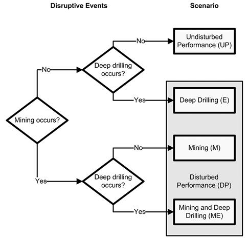
Figure PA- 4. Logic Diagram for Scenario Analysis

PA-2.3.2.1 Undisturbed Repository Performance

The UP scenario is defined in section 191.12 to mean "the predicted behavior of a disposal system, including consideration of the uncertainties in predicted behavior, if the disposal system is not disrupted by human intrusion or the occurrence of unlikely natural events." For compliance assessments with respect to the Individual and Groundwater Protection Requirements (section 191.15; Appendix IGP-2009), it is only necessary to consider the UP scenario. The UP scenario is also considered with DP scenario for PA with respect to the containment requirements (section 191.13).

No potentially disruptive natural events and processes are likely to occur during the regulatory time frame. Therefore, all naturally occurring events and processes retained for scenario construction are nondisruptive and are considered part of the UP scenario. Mining outside the LWB is assumed at the end of AIC for all scenarios. The mining scenario (M) involves future mining within the controlled area. The disturbed repository deep drilling scenario (E) involves at least one deep drilling event that intersects the waste disposal region. The M scenario and the E scenario may both occur in the future. The DOE calls a future in which both of these events occur the mining and drilling scenario (ME). More detailed descriptions are found in Section PA-2.3.2.2.

The potential effects of future deep drilling and/or mining within the controlled area are the only natural features and waste- (and repository-) induced FEPs retained after screening that are included in the DP scenario, but excluded in the UP scenario. Among the most significant FEPs that will affect the UP scenario within the disposal system are excavation-induced fracturing, gas generation, salt creep, and MgO in the disposal rooms.

· The repository excavation and consequent changes in the rock stress field surrounding the excavated opening will create a DRZ immediately adjacent to excavated openings. The DRZ will exhibit mechanical and hydrological properties different than those of the intact rock.

· Organic material in the waste may degrade because of microbial activity, and brine will corrode metals in the waste and waste containers, with concomitant generation of gases. Gas generation may result in pressures sufficient to both maintain or develop fractures and change the fluid flow pattern around the waste disposal region.

· At the repository depth, salt creep will tend to heal fractures and reduce the permeability of the DRZ, the crushed salt component of the shaft seals, and the ROM salt in the panel closures to near that of the host rock salt.

· The MgO engineered barrier emplaced in the disposal rooms will react with CO₂ and maintain mildly alkaline conditions. Metal corrosion in the waste and waste containers will maintain reducing conditions. These effects will maintain low radionuclide solubility.

Radionuclides can become mobile as a result of waste dissolution and colloid generation following brine flow into the disposal rooms. Colloids may be generated from the waste (humics, mineral fragments, microbes, and actinide intrinsic colloids) or from other sources (humics, mineral fragments, and microbes).

Conceptually, there are several pathways for radionuclide transport within the undisturbed disposal system that may result in releases to the accessible environment (Figure PA-5). Contaminated brine may migrate away from the waste-disposal panels if pressure within the panels is elevated by gas generated from corrosion or microbial consumption. Radionuclide transport may occur laterally, through the anhydrite interbeds toward the subsurface boundary of the accessible environment in the Salado, or through access drifts or anhydrite interbeds to the base of the shafts. In the latter case, if the pressure gradient between the panels and overlying strata is sufficient, contaminated brine may migrate up the shafts. As a result, radionuclides may be transported directly to the ground surface, or laterally away from the shafts through permeable strata such as the Culebra, toward the subsurface boundary of the accessible environment. These conceptual pathways are shown in Figure PA-5.

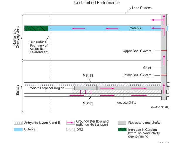
Figure PA- 5. Conceptual Release Pathways for the UP Scenario

The modeling system described in Section PA-4.0 includes potential radionuclide transport along other pathways, such as migration through Salado halite. However, the natural properties of the undisturbed system make radionuclide transport to the accessible environment via these other pathways unlikely.

PA-2.3.2.2 Disturbed Repository Performance

Assessments for compliance with section 191.13 need to consider the potential effects of future disruptive natural and human-initiated events and processes on the performance of the disposal system. No potentially disruptive natural events and processes are considered sufficiently likely to require inclusion in analyses of either the UP or DP scenario. The only future human-initiated events and processes retained after FEP screening are those associated with mining and deep drilling (but not the subsequent use of a borehole) within the controlled area or LWB when institutional controls cannot be assumed to eliminate the possibility of such activities (Section PA-3.2 and the CRA-2004, Chapter 6.0, Section 6.4.12.1). In total, 21 disturbed repository FEPs associated with future mining and deep drilling have been identified. These FEPs were assigned a screening designator of the DP scenario.

For evaluating the consequences of disturbed repository performance, the DOE has defined the M scenario, the E scenario, and the ME scenario. These scenarios are described in the following sections.

PA-2.3.2.2.1 Disturbed Repository M Scenario

The M scenario involves future mining within the controlled area. Consistent with the criteria stated by the EPA in section 194.32(b) for PA calculations, the effects of potential future mining within the controlled area are limited to changes in hydraulic conductivity of the Culebra that result from subsidence (as described in Section PA-3.9). The modeling system used for the M scenario is similar to that developed for the UP scenario, but with a modified Culebra T-field in the controlled area to account for the mining effects.

Radionuclide transport may be affected in the M scenario if a head gradient between the waste disposal panels and the Culebra causes brine contaminated with radionuclides to move from the waste disposal panels to the base of the shafts and up to the Culebra. The changes in the Culebra T-field may affect the rate and direction of radionuclide transport within the Culebra. Features of the M scenario are illustrated in Figure PA-6.

Three disturbed repository FEPs (H13, H37, and H57 in Appendix SCR-2004, Table SCR-1 ) are related to the occurrence and effects of future mining.

PA-2.3.2.2.2 Disturbed Repository E Scenario

The disturbed repository E scenario involves at least one deep drilling event that intersects the waste disposal region. The EPA provides criteria for analyzing the consequences of future drilling events in PA in section 194.33(c).

Performance assessments shall document that in analyzing the consequences of drilling events, the Department assumed that:

(1) Future drilling practices and technology will remain consistent with practices in the Delaware Basin at the time a compliance application is prepared. Such future drilling practices shall include, but shall not be limited to: the types and amounts of drilling fluids; borehole depths, diameters, and seals; and the fraction of such boreholes that are sealed by humans; and

(2) Natural processes will degrade or otherwise affect the capability of boreholes to transmit fluids over the regulatory time frame.

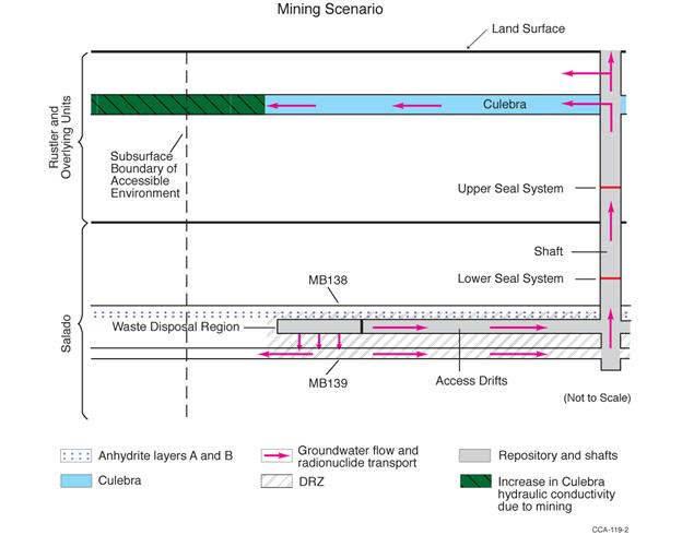
Figure PA- 6. Conceptual Release Pathways for the Disturbed Repository M Scenario

Consistent with these criteria, there are several pathways for radionuclides to reach the accessible environment in the E scenario. Before any deep drilling intersects the waste, potential release pathways are identical to those in the undisturbed repository scenario.

If a borehole intersects the waste in the disposal rooms, releases to the accessible environment may occur as material entrained in the circulating drilling fluid is brought to the surface. Particulate waste brought to the surface may include cuttings, cavings, and spallings. During drilling, contaminated brine may flow up the borehole and reach the surface, depending on fluid pressure within the waste disposal panels.

When abandoned, the borehole is assumed to be plugged in a manner consistent with current practices in the Delaware Basin as prescribed in section 194.33(c)(1). An abandoned intrusion borehole with degraded casing and/or plugs may provide a pathway for fluid flow and contaminant transport from the intersected waste panel to the ground surface if the fluid pressure within the panel is sufficiently greater than hydrostatic. Additionally, if brine flows through the borehole to overlying units, such as the Culebra, it may carry dissolved and colloidal actinides that can be transported laterally to the accessible environment by natural groundwater flow in the overlying units.

Alternatively, the units intersected by an intrusion borehole may provide sources for brine flow to a waste panel during or after drilling. For example, in the northern Delaware Basin, the Castile, which underlies the Salado, contains isolated volumes of brine at fluid pressures greater than hydrostatic (as discussed in the CRA-2004, Chapter 2.0, Section 2.2.1.2.2). The WIPP-12 borehole penetration of one of these volumes provided data on one pressurized brine pocket within the controlled area. The location and properties of brine pockets cannot be reliably predicted; thus, the possibility of a deep borehole penetrating both a waste panel and a brine reservoir is accounted for in consequence analysis of the WIPP, as discussed in the CRA-2004, Chapter 6.0, Section 6.4.8. Such a borehole could provide a connection for brine flow from the Castile to the waste panel, thus increasing fluid pressure and brine volume in the waste panel.

A borehole that is drilled through a disposal room pillar, but does not intersect waste, could also penetrate the brine reservoir underlying the waste disposal region. Such an event would, to some extent, depressurize the brine reservoir, and thus would affect the consequences of any subsequent reservoir intersections. The PA does not take credit for possible brine reservoir depressurization.

The DOE has distinguished two types of deep drilling events by whether or not the borehole intersects a Castile brine reservoir. A borehole that intersects a waste disposal panel and penetrates a Castile brine reservoir is designated an E1 event. A borehole that intersects a waste panel but does not penetrate a Castile brine reservoir is designated an E2 event. The consequences of deep drilling intrusions depend not only on the type of a drilling event, but on whether the repository was penetrated by an earlier E2 event or flooded due to an earlier E1 event. The PA also does not take credit for depressurization of brine reservoirs from multiple drilling intrusions. These scenarios are described in order of increasing complexity in the following sections.

PA-2.3.2.2.3 The E2 Scenario

The E2 scenario is the simplest scenario for inadvertent human intrusion into a waste disposal panel. In this scenario, a panel is penetrated by a drill bit; cuttings, cavings, spallings, and brine flow releases may occur; and brine flow may occur in the borehole after it is plugged and abandoned. Sources for brine that may contribute to long-term flow up the abandoned borehole are the Salado or, under certain conditions, the units above the Salado. An E2 scenario may involve more than one E2 drilling event, although the flow and transport model configuration developed for the E2 scenario evaluates the consequences of futures that have only one E2 event. Features of the E2 scenario are illustrated in Figure PA-7.

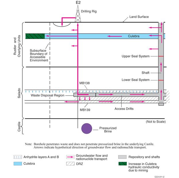
Figure PA- 7. Conceptual Release Pathways for the Disturbed Repository Deep Drilling E2 Scenario

PA-2.3.2.2.4 The E1 Scenario

Any scenario with exactly one inadvertent penetration of a waste panel that also penetrates a Castile brine reservoir is called E1. Features of this scenario are illustrated in Figure PA-8.

Sources of brine in the E1 scenario are the brine reservoir, the Salado, and, under certain conditions, the units above the Salado. However, the brine reservoir is conceptually the dominant source of brine in this scenario. The flow and transport model configuration developed for the E1 scenario evaluates the consequences of futures that have only one E1 event.

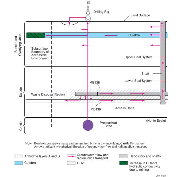
Figure PA- 8. Conceptual Release Pathways for the Disturbed Repository Deep Drilling E1 Scenario

PA-2.3.2.2.5 The E1E2 Scenario

The E1E2 scenario is defined as all futures with multiple penetrations of a waste panel of which at least one intrusion is an E1. One example of this scenario, with a single E1 event and a single E2 event penetrating the same panel, is illustrated in Figure PA-9. However, the E1E2 scenario can include many possible combinations of intrusion times, locations, and types of event (E1 or E2). The sources of brine in this scenario are those listed for the E1 scenario, and multiple E1 sources may be present. The E1E2 scenario has a potential flow path not present in the E1 or E2 scenarios: flow from an E1 borehole through the waste to another borehole. This flow path has the potential to (1) bring large quantities of brine in direct contact with waste and (2) provide a less restrictive path for this brine to flow to the units above the Salado (via multiple boreholes) compared to either the individual E1 or E2 scenarios. It is both the presence of brine reservoirs and the potential for flow through the waste to other boreholes that make this scenario different from combinations of E2 boreholes in terms of potential consequences.

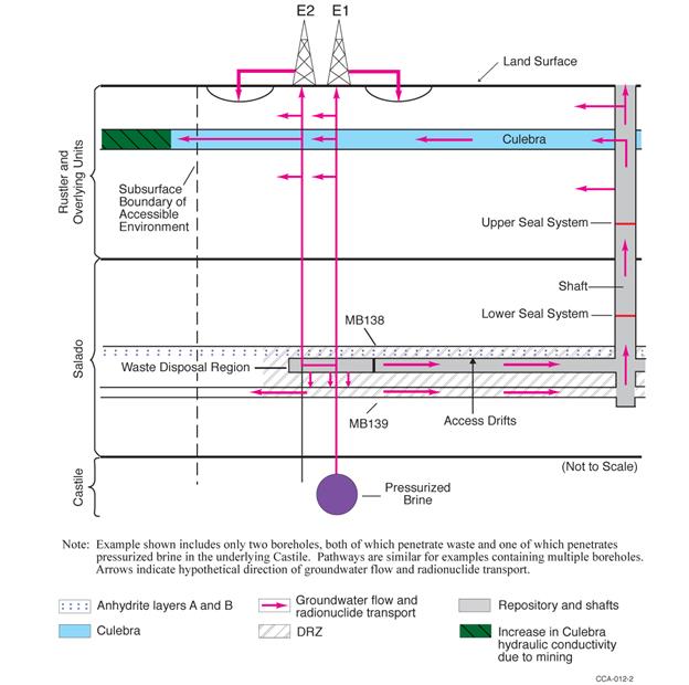
Figure PA- 9. Conceptual Release Pathways for the Disturbed Repository Deep Drilling E1E2 Scenario

PA-2.3.2.3 Disturbed Repository ME Scenario

The M scenario and the E scenario may both occur in the future. The DOE calls a future in which both of these events occur the ME scenario. The occurrence of both mining and deep drilling do not create processes beyond those already described separately for the M and E scenarios. For example, the occurrence of mining does not influence any of the interactions between deep boreholes and the repository or brine reservoirs, nor does the occurrence of drilling impact the effects of mining on Culebra hydrogeology.

PA-2.3.2.4 Scenarios Retained for Consequence Analysis

The scenarios described in Section PA-2.3.2.1, Section PA-2.3.2.2, and Section PA-2.3.2.3 have been retained for consequence analysis to determine compliance with the containment requirements in section 191.13. The modeling systems used to evaluate the consequences of these undisturbed and disturbed scenarios are discussed in Section PA-2.3.3.

PA-2.3.3 Calculation of Scenario Consequences

Calculating scenario consequences requires quantitative modeling. This section discusses the conceptual and computational models and some parameter values used to estimate the consequence of the scenarios described in Section PA-2.3.2. Additional discussion of conceptual models and modeling assumptions is provided in Section PA-4.0. Additional descriptions of sampled parameter values are included in Kicker and Herrick (Kicker and Herrick 2013).

A single modeling system was used to represent the disposal system and calculate the CCDFs. The modeling system, however, can be conveniently described in terms of various submodels, with each describing a part of the overall system. The models used in the WIPP PA, as in other complex analyses, exist at four different levels.

1. Conceptual models are a set of qualitative assumptions that describe a system or subsystem for a given purpose. At a minimum, these assumptions concern the geometry and dimensionality of the system, initial and boundary conditions, time dependence, and the nature of the relevant physical and chemical processes. The assumptions should be consistent with one another and with existing information within the context of the given purpose.

2. Mathematical models represent the processes at the site. The conceptual models provide the context within which these mathematical models must operate, and define the processes they must characterize. The mathematical models are predictive in the sense that, once provided with the known or assumed properties of the system and possible perturbations to the system, they predict the response of the system. The processes represented by these mathematical models include fluid flow, mechanical deformation, radionuclide transport in groundwater, and removal of waste through intruding boreholes.

3. Numerical models are developed to approximate mathematical model solutions because most mathematical models do not have closed-form solutions.

4. Computational models generally refer to the implementation of the numerical models in the computer code with specific initial and boundary conditions and parameter values. The complexity of the system requires computer codes to solve the numerical models.

Parameters are values necessary in mathematical, numerical, or computational models. Data are descriptors of the physical system being considered, normally obtained by experiment or observation. The distinction between data and parameters can be subtle. Parameters are distinct from data, however, for three reasons: (1) Data may be evaluated, statistically or otherwise, to generate model parameters to account for uncertainty in data. (2) Some parameters have no relation to the physical system, such as the parameters in a numerical model to determine when an iterative solution scheme has converged. (3) Many model parameters are applied at a different scale than one directly observed or measured in the physical system. The distinction between data and parameter values is described further in Kicker and Herrick (Kicker and Herrick 2013) and Tierney (Tierney 1990), where distribution derivations for specific parameters are given.

PA-3.0 Probabilistic Characterization of Futures

The PA for the WIPP identifies uncertainty in parameters and uncertainty in future events as distinctly different entities and requires sampling to be conducted in two dimensions. One dimension focuses on characterizing the uncertainty in terms of the probability that various possible futures will occur at the WIPP site over the next 10,000 years. The other dimension characterizes the uncertainty due to lack of knowledge about the precise values of model parameters appropriate for the WIPP repository. Each dimension of the analysis is characterized by a probability space. Monte Carlo methods are used with the WIPP PA modeling system to sample each of the two probability spaces.

Characterizing the probability distribution for the first dimension of the PA depends on identifying the kinds of events that could impact releases from the repository over the next 10,000 years. Screening analyses of possible future events concluded that the only significant events with the potential to affect radionuclide releases to the accessible environment are drilling and mining within the LWB (Appendix SCR-2004, Section SCR-5.0 ). Consequently, modeling the future states of the repository focuses on representing the occurrences and effects of these two events. CCDFGF uses stochastic processes to simulate intrusion events by drilling and the occurrence of mining for natural resources. CCDFGF assembles the results from the deterministic models and selects the most appropriate scenario data provided by these models to use as the simulation of a 10,000-year future progresses. Ten thousand potential futures are simulated and used to create distributions of potential releases, and then compiled into a single CCDF of potential releases.

The WIPP PA is required not only to estimate the likelihood of future releases, but to establish statistical confidence in those estimates. Confidence is established using the second dimension of the analysis, which is based on the evaluation of uncertainty in the values of some of the parameters of the deterministic models. This uncertainty is assumed to represent a lack of knowledge about the true values of the parameters, and is labeled epistemic uncertainty. Epistemic uncertainty can be viewed as the representation of potential systematic errors in the results. The impact of epistemic uncertainty on the results is determined by generating 300 sets of parameter values using a stratified random sampling design, LHS, and then running the deterministic models and CCDFGF with each set of sampled parameters. Thus, 300 CCDFs are generated by CCDFGF. The 300 simulations are organized as 3 replicates of 100 vectors each. Because the uncertainty assigned to the parameters represents a lack of knowledge, this epistemic uncertainty could theoretically be reduced by collecting data to improve knowledge about the parameters. Epistemic uncertainty is represented in the projections of potential releases from the repository by the variability among the 300 CCDFs.

The WIPP PA modeling system consists of a set of coupled deterministic models (BRAGFLO, PANEL, NUTS, SECOTP2D, and CUTTINGS_S) that provide scenario-specific results to the code CCDFGF (Figure PA-1). CCDFGF is, in contrast, a stochastic simulation model used to simulate potential futures of repository performance where drilling and mining intrusions can impact the state of the repository and produce release events. CCDFGF implements the timing of intrusions as stochastic events, thus incorporating the aleatory uncertainty associated with projections of future events. This section describes how aleatory uncertainty is implemented in PA. Epistemic uncertainty is discussed in Section PA-6.0.

PA-3.1 Probability Space

As discussed in Section PA-2.2.2, aleatory uncertainty is defined by the possible futures x _st,i conditional on the set i of parameters used in Equation (PA.2). Section PA-3.2, Section PA-3.3, Section PA-3.4, Section PA-3.5, Section PA-3.6, Section PA-3.7, Section PA-3.8, and Section PA-3.9 describe the individual components t _j , e _j , l _j , b _j , p _j , a _j , and t _min of x _st,i and their associated probability distributions. The concept of a scenario as a subset of the sample space of x _st,i is discussed in Section PA-3.10. The procedure used to sample the individual elements x _st,i is described in Section PA-6.5.

PA-3.2 AICs and PICs

The AICs and PICs will be implemented at the WIPP site to deter human activity detrimental to repository performance. The AICs and PICs are described in detail in the CRA-2004, Chapter 7.0 and in appendices referenced in Chapter 7.0. Permanent markers will be constructed to inform future populations of the location of the WIPP, and part of the marker system will be a berm that defines the active areas of the repository. In this section, the impact of AICs and PICs on PA is described.

The AICs will be implemented at the WIPP after final facility closure to control site access and ensure that activities detrimental to disposal system performance do not occur within the controlled area. The AICs will preclude human intrusion in the disposal system. A 100-year limit on the effectiveness of AICs in PA is established in section 191.14 (a). Because of the regulatory restrictions and the nature of the AICs that will be implemented, PA assumes there are no inadvertent human intrusions or mining in the controlled area for 100 years following repository closure.

The PICs are designed to deter inadvertent human intrusion into the disposal system. Only minimal assumptions were made about the nature of future society when designing the PICs to comply with the assurance requirements. The preamble to Part 194 limits any credit for PICs in deterring human intrusion to 700 years after disposal (U.S. EPA 1996a, p. 5231). Although the DOE originally took credit for PICs in the CCA PA, it has not taken credit since. Not including PICs is a conservative implementation, as no credit is taken for a beneficial component of the system.

PA-3.3 Drilling Intrusion

As described in Section PA-2.3.2.2, drilling intrusions in PA are assumed to occur randomly in time and space following a Poisson process. Specifically, the drilling rate considered within the area marked by a berm as part of the system for PICs (Kicker and Herrick 2013, Table 38) is 6.73 ´ 10^-3 intrusions per square kilometer per year (km^- ² yr^-1). AICs are assumed to prevent any drilling intrusions for the first 100 years after the decommissioning of the WIPP (Section PA-3.2). In the computational implementation of PA, it is convenient to represent the Poisson process for drilling intrusions by its corresponding rate term l _d (t) for intrusions into the area marked by the berm. Specifically,

(PA.6)

where 0.6285 km² is the area enclosed by the berm (Kicker and Herrick 2013, Table 37) and t is the elapsed time (in years) since decommissioning the WIPP.

The function l _d (t) defines the parameter of the exponential distribution that gives rise to the times of intrusions, t _j of Equation (PA.2). In the computational implementation of the analysis, the exponential distribution is randomly sampled to define the times between successive drilling intrusions (Figure PA-10 and Section PA-6.5). A key assumption of the exponential distribution is that events are independent of each other, so the occurrence of one event has no effect on the occurrence of the next event. The process giving rise to such events is sometimes called a Poisson process because the distribution of such events over a fixed interval of time is a Poisson distribution. Due to the 10,000-year regulatory period specified in section 191.13, t _j is assumed to be bounded above by 10,000 years in the definition of x _st,i . Further, t _j is bounded below by 100 years as defined in Equation (PA.6).

Figure PA- 10. CDF for Time Between Drilling Intrusions

PA-3.4 Penetration of Excavated/Nonexcavated Area

The variable e _j is a designator for whether or not the j ^th drilling intrusion penetrates an excavated, waste-filled area of the repository: e _j = 0 or 1 implies penetration of a nonexcavated or excavated area, respectively. The corresponding probabilities P[e _j = 0] and P[e _j = 1] for e _j = 0 and e _j = 1 are

(PA.7)

(PA.8)

where 0.1273 km² and 0.6285 km² are the excavated area of the repository and the area of the berm, respectively (Kicker and Herrick 2013, Table 37).

PA-3.5 Drilling Location

Locations of drilling intrusions through the excavated, waste-filled area of the repository are discretized to the 144 locations in Figure PA-11. Assuming that a drilling intrusion occurs within the excavated area, it is assumed to be equally likely to occur at each of these 144 locations. Thus, the probability pL _k that drilling intrusion j will occur at location l _k , k = 1, 2, ¼, 144 in Figure PA-11 is

(PA.9)

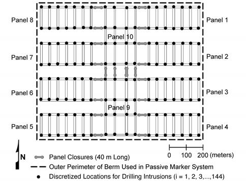
Figure PA- 11. Discretized Locations for Drilling Intrusions

PA-3.6 Penetration of Pressurized Brine

The conceptual models for the Castile include the possibility that pressurized brine reservoirs underlie the repository (Section PA-4.2.10). The variable b _j is a designator for whether or not the j ^th drilling intrusion penetrates pressurized brine, where b _j = 0 signifies nonpenetration and b _j = 1 signifies penetration of pressurized brine. In the CRA-2014 PA, the probability of encountering pressurized brine during a drilling intrusion has been refined from that used in the CRA-2009 PABC. Specifically, the probability pB ₁ = P[b _j = 1] in the CRA-2014 PA is sampled from a normal distribution ranging from 0.06 to 0.19 (see Section PA-1.1.3 and Kirchner et al. 2012).

PA-3.7 Plugging Pattern

Three borehole plugging patterns, p _k , are considered in PA: (1) p ₁ , a full concrete plug through the Salado to the Bell Canyon Formation (hereafter referred to as Bell Canyon), (2) p ₂, a two-plug configuration with concrete plugs at the Rustler/Salado interface and the Castile/Bell Canyon interface, and (3) p ₃ , a three-plug configuration with concrete plugs at the Rustler/ Salado, Salado/Castile, and Castile/Bell Canyon interfaces. The DOE continues to survey drilling activity in the Delaware Basin in accordance with the criteria established in section 194.33. Results for the year 2012 are documented in the 2012 Delaware Basin Monitoring Annual Report (U.S. DOE 2012). Drilling parameters are updated in the CRA-2014 PA to include information assembled through year 2012. The probability that a given drilling intrusion will be sealed with plugging pattern p _k , k= 1, 2, 3, is given by pPL _k , where pPL ₁ = P[k = 1] = 0.04, pPL ₂ = P[k = 2] = 0.594, pPL ₃ = P[k = 3] = 0.366 (Kicker and Herrick 2013, Table 38).

PA-3.8 Activity Level

The waste intended for disposal at the WIPP is represented by 528 distinct waste streams, with 451 of these waste streams designated as CH-TRU waste and 77 designated as RH-TRU waste (Kicker and Zeitler 2013a). For the CRA-2014 PA, the 77 separate RH-TRU waste streams are represented by a single, combined RH-TRU waste stream, as has been done in all previous PAs. The activity levels for the waste streams are given in Kicker and Herrick 2013, Tables B-1 and B-2. Each waste container emplaced in the repository contains waste from a single CH-TRU waste stream. Waste packaged in 55-gallon (gal) drums is stacked 3 drums high within the repository. Although waste in other packages (e.g., standard waste boxes, 10-drum overpacks, etc.) may not be stacked 3 high, PA assumes that each drilling intrusion into CH-TRU waste intersects 3 different waste streams. In contrast, all RH-TRU waste is represented by a single waste stream, and so each drilling intrusion through RH-TRU waste is assumed to intersect this single waste stream. Appendix MASS-2014, Section MASS-19.0 examines the sensitivity of PA results to the assumption that three waste streams are intersected by each drilling intrusion into CH-TRU waste.

The vector a _j characterizes the type of waste penetrated by the j ^th drilling intrusion. Specifically,

a _j = 0 if e j = 0 (PA.10)

(i.e., if the i ^th drilling intrusion does not penetrate an excavated area of the repository)

a _j = 1 if e_j = 1 and RH-TRU is penetrated (PA.11)

a _j = [iCH_j1 , iCH_j2 , iCH_j3 ] if e_j = 1 and CH-TRU is penetrated (PA.12)

where iCH _j1 , iCH _j2 , and iCH _j3 are integer designators for the CH-TRU waste streams intersected by the j ^th drilling intrusion (i.e., each of iCH _j1 , iCH _j2 , and iCH _j3 is an integer between 1 and 451).

Whether the j ^th intrusion penetrates a nonexcavated or excavated area is determined by the probabilities pE ₀ and pE ₁ discussed in Section PA-3.4. The type of waste penetrated is determined by the probabilities pCH and pRH. The excavated area used for disposal of CH-TRU waste (aCH) is 1.115 ´ 10⁵ square meters (m²) and the area used for disposal of RH-TRU waste (aRH) is 1.576 ´ 10⁴ m² (Kicker and Herrick 2013, Table 37), for a total disposal area of aEX = aCH + aRH = 1.273 ´ 10⁵ m². Given that the j ^th intrusion penetrates an excavated area, the probabilities pCH and pRH of penetrating CH-TRU and RH-TRU waste are given by

(PA.13)

(PA.14)

As indicated in this section, the probabilistic characterization of a _j depends on a number of individual probabilities. Specifically, pEx ₀ and pEx ₁ determine whether a nonexcavated or excavated area is penetrated (Section PA-3.5). Probabilities pCH and pRH determine whether CH-TRU or RH-TRU waste is encountered, given penetration of an excavated area. The individual waste stream volumes in Kicker and Herrick (Kicker and Herrick 2013), Tables B-1 and B-2 are used to determine the specific waste streams iCH _j1 , iCH _j2 , and iCH _j3 encountered, given a penetration of CH-TRU waste. The probability of encountering a particular CH-TRU waste stream is computed as the ratio of the volume of that waste stream to the volume of CH-TRU waste.

PA-3.9 Mining Time

Full mining of known potash reserves within the LWB is assumed to occur at time t _min . The occurrence of mining within the LWB in 10,000 years in the absence of institutional controls is specified as following a Poisson process with a rate of l _m = 1 ´ 10^- ⁴ yr^- ¹ (parameter GLOBAL:MINERT in Kicker and Herrick 2013, Table 38). However, this rate can be reduced by AICs and PICs. Specifically, AICs are assumed to result in no possibility of mining for the first 100 years after decommissioning of the WIPP. In PA, PICs do not affect the mining rate. Thus, the mining rate l _m (t) is

(PA.15)

(PA.16)

where t is the elapsed time since decommissioning of the WIPP.

In the computational implementation of the analysis, l _m (t) is used to define the distribution of time to mining. The use of l _m (t) to characterize t _min is analogous to the use of l _d to characterize the t _j , except that only one mining event is assumed to occur (i.e., x _st, _i contains only one value for t _min ) in order to be consistent with guidance given in Part 194 that mining within the LWB should be assumed to remove all economically viable potash reserves. Due to the 10,000-year regulatory period specified in section 191.13, t _min is assumed to be bounded above by 10,000 years in the definition of x _st,i .

PA-3.10 Scenarios and Scenario Probabilities

A scenario is a subset of the sample space for aleatory uncertainty. The underlying goal of scenario definition is to define the state of repository conditions prior to and following intrusion events. Scenarios are specific cases of inputs or system states that are selected to cover the range of possible cases. Given the complexity of the futures x _st,i (see Equation (PA.2)), many different scenarios can be defined. The computational complexity of the function f(x _st |v _su ) in Section PA-2.2.3 limits evaluation to only a few intrusion scenarios. As presented in Section PA-2.3.2, PA considers four fundamental intrusion scenarios:

E0 = no drilling intrusion through an excavated area of the repository

E1 = a drilling intrusion through an excavated area of the repository that penetrates pressurized brine in the Castile

E2 = a drilling intrusion through an excavated area of the repository that does not penetrate pressurized brine in the Castile

E1E2 = two or more previous intrusions, at least one of which is an E1 intrusion

These definitions of intrusion scenarios capture the most important events impacting the state of the repository: whether or not the repository is inundated by the penetration of a brine pocket, and whether or not there exists a possible route of release upward via a borehole. The state of the repository is also designated as E0, E1, E2, or E1E2. Scenarios for some of the process-level models consist of a single intrusion scenario occurring at specific times. CCDFGF is used to simulate multiple intrusions over 10,000 years (see section PA-3.11).

If only the intrusion scenarios controlled the state of the repository, then the state would be defined by the sequence of drilling events alone. However, CCDFGF also considers the impact of plugging pattern on boreholes. A borehole with a full plugging pattern that penetrates the waste area is also assumed to have no impact, and leaves the repository in its previous state, including the undisturbed state (see Section PA-6.8.4.1 and Figure PA-33 for more details). Thus, an E2 intrusion event into an E0 repository will result in an E0 state if a full plugging pattern is used, or an E2 state otherwise. An E1 intrusion subsequent to an E2 intrusion will leave the repository in an E1E2 state, where it will remain, regardless of subsequent intrusions. It is therefore important to distinguish between the type of intrusion, listed above, and the state of the repository.

The probability that no excavated area will be penetrated during the 10,000-year interval can be computed using a distribution of the number of penetration events and the probability that a drilling event will penetrate the excavated area. For the Poisson distribution of drilling events, the probability of there being n events in the 10,000-year history is

(PA.17)

where l _d is the mean drilling rate per year in the period following the period of AICs, 9,900 is the number of years in which drilling can occur after the institutional control period of 100 years, and n is the number of drilling events. The probability of having n events all within the nonexcavated area is pEx ₀ ⁿ, or specifically 0.797ⁿ. Thus, the probability of having only events in the nonexcavated area over 10,000 years, i.e., having no drilling intrusions into the excavated area, is just the sum across all n of the products of the probability of having exactly n drilling events and the probability that all n events penetrate the unexcavated area:

(PA.18)

The calculated probability becomes

exp[-0.203(4.23×10^-3)(10000-100)] = 2.03×10^-4 (PA.19)

This probability is the lower bound on the probability of the repository being in an E0 state, given that it does not include the consideration of the plugging pattern.

The probability of a single E1, E2, or E1E2 intrusion over 10,000 years is relatively small. Assuming that pB ₁ takes on its mean value of 0.127 (see Section PA-3.6), and ignoring the impact of the plugging pattern, for a constant rate of drilling, l _d , these equations are

exp[-9900 𝝀 _d pEx₁ ](9900 𝝀 _d pEx₁ )pB₁ = 2.2×10^-4 (PA.20)

and

exp[-9900 𝝀 _d pEx₁ ](9900 𝝀 _d pEx₁ )pB₀ = 1.5×10^-3 (PA.21)

respectively, where (pEx ₁ × l _d ) represents the annual rate of drilling into the excavated region of the repository which is multiplied by 9900 to give the frequency per 9,900 years. The probability of an intrusion into the excavated area is subsequently multiplied by the probability of hitting or missing a brine pocket. In this form, it can be seen that the term for the probability for intrusion is equivalent to the PDF of the Poisson distribution for n = 1:

(PA.22)

The expressions defining the probability of being in the E0 state after 10,000 years and of having a single E1 or E2 intrusion event after 10,000 years are relatively simple because the scenarios E0, E1, and E2 are relatively simple. The scenario E1E2 is more complex and, as a result, computing its probability is also more complex. Closed-form formulas for the probabilities of quite complex scenarios can be derived, but they are very complicated and involve large numbers of iterated integrals (Helton 1993).

PA-3.11 CCDF Construction

CCDFGF simulates histories that can have many intrusion events (WIPP Performance Assessment 2010). The process-level models evaluate the releases at a small number of specific times for each of the four intrusion scenarios. Releases from the repository are calculated using results from these fundamental scenarios (Section PA-6.7 and Section PA-6.8). Releases for an arbitrary future are estimated from the results of these fundamental scenarios (Section PA-6.8); these releases are used to construct CCDFs by Equation (PA.4).

The WIPP PA uses the Monte Carlo approach to construct the CCDF indicated in Equation (PA.4). The Monte Carlo approach generates releases for 10,000 possible futures. CCDFs are constructed by treating the 10,000 releases values as order statistics; each release is assigned a probability of 1 ´ 10^-4, and the CCDF can be constructed by plotting the complement of the sum of the probabilities ordered by the release value. The CRA-2014 PA uses the same approach as the CRA-2009 PA.

PA-4.0 Estimation of Releases

This section describes how releases to the accessible environment are estimated for a particular future in PA.

PA-4.1 Results for Specific Futures

The function f(x _st,i ) estimates the radionuclide releases to the accessible environment associated with each of the possible futures (x _st,i ) that could occur at the WIPP site over the next 10,000 years. In practice, f(x _st,i ) is quite complex and is constructed by the models implemented in computer programs used to simulate important processes and releases at the WIPP. In the context of these models, f(x _st,i ) has the form

(PA.23)

where

x _st,i ~ particular future under consideration

~ future involving no drilling intrusions but a mining event at the same time t _min as in x _st

f _C(x _st,i ) ~ cuttings and cavings release to accessible environment for x _st,i calculated with CUTTINGS_S

f _B(x _st,i ) ~ two-phase flow in and around the repository calculated for x _st,i with BRAGFLO; in practice, f _B (x _st,i ) is a vector containing a large amount of information, including pressure and brine saturation in various geologic members

~ spallings release to accessible environment for x _st,i calculated with the spallings model contained in DRSPALL and CUTTINGS_S; this calculation requires repository conditions calculated by f _B (x _st,i ) as input

~ DBR to accessible environment for x _st,i also calculated with BRAGFLO; this calculation requires repository conditions calculated by f _B (x _st,i ) as input

~ release through anhydrite MBs to accessible environment for x _st,i calculated with NUTS; this calculation requires flows in and around the repository calculated by f _B (x _st,i ) as input

~ release through Dewey Lake to accessible environment for x _st,i calculated with NUTS; this calculation requires flows in and around the repository calculated by f _B (x _st,i ) as input

~ release to land surface due to brine flow up a plugged borehole for x _st,i calculated with NUTS; this calculation requires flows in and around the repository calculated by f _B (x _st,i ) as input

~ flow field in the Culebra calculated for x _st, ₀ with MODFLOW; x _st, ₀ is used as an argument to f _MF because drilling intrusions are assumed to cause no perturbations to the flow field in the Culebra

~ release to Culebra for x _st,i calculated with NUTS or PANEL as appropriate; this calculation requires flows in and around the repository calculated by f _B (x _st,i ) as input

~ groundwater transport release through Culebra to accessible environment calculated with SECOTP2D. This calculation requires MODFLOW results (i.e., f _MF (x _st,0 )) and NUTS or PANEL results (i.e., ) as input

The remainder of this section describes the mathematical structure of the mechanistic models that underlie the component functions of f(x _st,i ) in Equation (PA.23).

The Monte Carlo CCDF construction procedure, implemented in the code CCDFGF (WIPP Performance Assessment 2010), uses a sample of size nS = 10,000 in PA. The individual programs that estimate releases do not run fast enough to allow this many evaluations of f. As a result, a two-step procedure is being used to evaluate f in calculating the summation in Equation (PA.23). First, f and its component functions are evaluated with the procedures (i.e., models) described in this section for a group of preselected futures. Second, values of f(x _st ) for the randomly selected futures x _st,i used in the numerical evaluation of the summation in Equation (PA.23) are then constructed from results obtained in the first step. These constructions are described in Section PA-6.7 and Section PA-6.8, and produce the evaluations of f(x _st ) that are actually used in Equation (PA.23).

For notational simplicity, the functions on the right-hand side of Equation (PA.23) will typically be written with only x _st as an argument (e.g., f _SP (x _st ) and will be used instead of f _SP [x _st , f _B (x _st )]). However, the underlying dependency on the other arguments will still be present.

The major topics considered in this chapter are two-phase flow in the vicinity of the repository as modeled by BRAGFLO (i.e., f _B ) (Section PA-4.2), radionuclide transport in the vicinity of the repository as modeled by NUTS (i.e., f _MB , f _DL , f _S , f _NP ) (Section PA-4.3), radionuclide transport in the vicinity of the repository as modeled by PANEL (i.e., f _NP ) (Section PA-4.4), cuttings and cavings releases to the surface as modeled by CUTTINGS_S (i.e., f _C ) (Section PA-4.5), spallings releases to the surface as modeled by DRSPALL and CUTTINGS_S (i.e., f _SP ) (Section PA-4.6), DBRs to the surface as modeled by BRAGFLO (i.e., f _DBR ) (Section PA-4.7), brine flow in the Culebra as modeled by MODFLOW (i.e., f _MF ) (Section PA-4.8), and radionuclide transport in the Culebra as modeled by SECOTP2D (i.e., f _ST ) (Section PA-4.9).

PA-4.2 Two-Phase Flow: BRAGFLO

Quantifying the effects of gas and brine flow on radionuclide transport from the repository requires a two-phase (brine and gas) flow code. The two-phase flow code BRAGFLO is used to simulate gas and brine flow in and around the repository (Camphouse 2013a and Camphouse 2013b). Additionally, the BRAGFLO code incorporates the effects of disposal room consolidation and closure, gas generation, and rock fracturing in response to gas pressure. This section describes the mathematical models on which BRAGFLO is based, the representation of the repository in the model, and the numerical techniques employed in the solution.

PA-4.2.1 Mathematical Description

Two-phase flow in the vicinity of the repository is represented by the following system of two conservation equations, two constraint equations, and three equations of state:

Gas Conservation

Ñ × (PA.24)

Brine Conservation

Ñ × (PA.25)

Saturation Constraint

(PA.26)

Capillary Pressure Constraint

(PA.27)

Gas Density

r _g (determined by Redlich-Kwong-Soave (RKS) equation of state; see Equation (PA.51))
(PA.28)

Brine Density

(PA.29)

Formation Porosity

(PA.30)

where

g = acceleration due to gravity (meters per second squared [m])

h = vertical distance from a reference location (m)

k rl = relative permeability (dimensionless) to fluid l, l = b (brine), g (gas)

P _c = capillary pressure in Pascals (Pa)

P _l = pressure of fluid l (Pa)

q rl = rate of production (or consumption, if negative) of fluid l due to chemical reaction (kilograms per cubic meter per seconds [kg/m³/s])

q _l = rate of injection (or removal, if negative) of fluid l (kg/m³/s)

S l = saturation of fluid l (dimensionless)

t = time (s)

a = geometry factor (m)

r l = density of fluid l (kg/m³)

m l = viscosity of fluid l (Pa s)

f = porosity (dimensionless)

f 0 = reference (i.e., initial) porosity (dimensionless)

P b 0 = reference (i.e., initial) brine pressure (Pa), constant in Equation (PA.29) and spatially variable in Equation (PA.30)

r 0 = reference (i.e., initial) brine density (kg/m³)

c _f = pore compressibility (Pa^-1)

c _b = brine compressibility (Pa^-1)

K = permeability of the material (m²), isotropic for PA (Howarth and Christian-Frear 1997)

For the brine transport Equation (PA.25), the intrinsic permeability of the material is used. For the gas transport Equation (PA.24), the permeability K is modified to account for the Klinkenberg effect (Klinkenberg 1941). Specifically,

(PA.31)

where a and b are gas and formation-dependent constants. Values of a = -0.3410 and b = 0.2710 were determined from data obtained for MB 139 (Christian-Frear 1996), with these values used for all material regions in Figure PA-12.

The conservation equations are valid in one (i.e., Ñ = [ ¶ / ¶ x]), two (i.e., Ñ = [ ¶ / ¶ x, ¶ / ¶ y]), and three (i.e., Ñ = [ ¶ / ¶ x, ¶ / ¶ y, ¶ / ¶ z]) dimensions. In PA, the preceding system of equations is used to model two-phase fluid flow within the two-dimensional region shown in Figure PA-12. The details of this system are discussed below.

The a term in Equation (PA.24) and Equation (PA.25) is a dimension-dependent geometry factor and is specified by

a = area normal to flow direction in one-dimensional flow (i.e., D y D z; units = m²)

= thickness normal to flow plane in two-dimensional flow (i.e., D z; units = m)

= 1 in three-dimensional flow (dimensionless) (PA.32)

PA uses a two-dimensional geometry to compute two-phase flow in the vicinity of the repository, and as a result, a is the thickness of the modeled region (i.e., D z) normal to the flow plane (Figure PA-12). Due to the use of the two-dimensional grid in Figure PA-12, a is spatially dependent, with the values used for a defined in the column labeled "D z." Specifically, a increases with distance away from the repository edge in both directions to incorporate the increasing pore volume through which fluid flow occurs. The method used in PA, called rectangular flaring, is illustrated in Figure PA-13 and ensures that the total volume surrounding the repository is conserved in the numerical grid. The equations and method used to determine a for BRAGFLO grids used in the WIPP PA were developed by Stein (Stein 2002).

The h term in Equation (PA.24) and Equation (PA.25) defines vertical distance from a reference point. In PA, this reference point is taken to be the center of MB 139 at the location of the shaft (i.e., (x _ref , y _ref ) = (23664.9 m, 378.685 m), which is the center of cell 1272 in Figure PA-14). Specifically, h is defined by

(PA.33)

where q is the inclination of the formation in which the point (x, y) is located. In PA, the Salado is modeled as having an inclination of 1 degree from north to south, and all other formations are modeled as being horizontal. Thus, q = 1 degree for points within the Salado, and q = 0 degrees otherwise. Treating the Salado as an inclined formation and treating the Castile, Castile brine reservoir, Rustler, and overlying units as horizontal creates discontinuities in the grid at the lower and upper boundaries of the Salado. However, this treatment does not create a computational problem, since the Salado is isolated from vertical flow; its upper boundary adjoins the impermeable Los Medaños Member (formerly referred to as the Unnamed Member) at the base of the Rustler, and its lower boundary adjoins the impermeable Castile.

In the solution of Equation (PA.24), Equation (PA.25), Equation (PA.26), Equation (PA.27), Equation (PA.28), Equation (PA.29) and (PA.30), S _b and S _g are functions of location and time. Thus, P _c , k _rb , and k _rg are functions of the form P _c (x, y, t), k _rb (x, y, t), and k _rg (x, y, t). In the computational implementation of the solution of the preceding equations, flow of phase l out of a computational cell (Figure PA-14) cannot occur when S _l (x, y, t) £ S _lr (x, y, t), where S _lr denotes the residual saturation for phase l. The values used for S _lr , l = b, g are summarized in Table PA-3.

	Table PA-3. Parameter Values Used in Representation of Two-Phase Flow (Continued)

Region	Material	Material Description	Brooks-Corey Pore Distribution (PORE_DIS)^a l	Threshold Pressure Linear Parameter (PCT_A)^a a	Threshold Pressure Exponential Parameter (PCT_EXP)^a h	Residual Brine Saturation (SAT_RBRN)^a Sbr	Residual Gas Saturation (SAT_RGAS)^a Sgr	Porosity (POROSITY)^a f 0	Pore Compressibility^a c f , Pa^-1	Intrinsic Permeability (PRMX_LOG)^a k, m²
Salado	S_HALITE	Undisturbed halite	0.7	0.56	- 0.346	0.3	0.2	HALPOR^b	f(HALCOMP)^b,d	10^x, x = HALPRM^b
DRZ	DRZ_0	DRZ, - 5 to 0 years	0.7	0.0	0.0	0.0	0.0	f(HALPOR)^b,c	f(HALCOMP)^b,d	1.0 ´ 10-17
DRZ_1	DRZ, 0 to 10,000 years	0.7	0.0	0.0	0.0	0.0	f(HALPOR)^b,c	f(HALCOMP)^b,d	10^x, x = DRZPRM^b
MB 138	S_MB138	Anhydrite MB in Salado	ANHBCEXP^b	0.26	- 0.348	ANRBSAT^b	ANRGSSAT^b	0.011	f(ANHCOMP)^b,d	10^x, x = ANHPRM^b
Anhydrite AB	S_ANH_AB	Anhydrite layers A and B in Salado	ANHBCEXP^b	0.26	- 0.348	ANRBSAT^b	ANRGSSAT^b	0.011	f(ANHCOMP)^b,d	10^x, x = ANHPRM^b
MB 139	S_MB139	Anhydrite MB in Salado	ANHBCEXP^b	0.26	- 0.348	ANRBSAT^b	ANRGSSAT^b	0.011	f(ANHCOMP)^b,d	10^x, x = ANHPRM^b
Waste Panel	CAVITY_1	Single waste panel, - 5 to 0 years	NA^e	NA^e	NA^e	0.0	0.0	1.0	0.0	1.0 ´ 10 ^- ¹⁰
WAS_AREA	Single waste panel, 0 to 10,000 years	2.89	0.0	0.0	WRBRNSAT^b	WRGSSAT^b	0.848^f	0.0	2.4 ´ 10 ^- ¹³
Rest of Repository (SRoR and NRoR)	CAVITY_2	RoR, - 5 to 0 years	NA^e	NA^e	NA^e	0.0	0.0	1.0	0.0	1.0 ´ 10 ^- ¹⁰
REPOSIT	RoR, 0 to 10,000 years	2.89	0.0	0.0	WRBRNSAT^b	WRGSSAT^b	0.848^f	0.0	2.4 ´ 10 ^- ¹³
Ops	CAVITY_3	Operations area, - 5 to 0 years	NA^e	NA^e	NA^e	0.0	0.0	1.0	0.0	1.0 ´ 10 ^- ¹⁰
OPS_AREA	Operations area, 0 to 10,000 years	NA^e	NA^e	NA^e	0.0	0.0	0.18	0.0	1.0 ´ 10 ^- ¹¹
Exp	CAVITY_3	Experimental area, - 5 to 0 years	NA^e	NA^e	NA^e	0.0	0.0	1.0	0.0	1.0 ´ 10 ^- ¹⁰
	a Parenthetical parameter names are property names for the corresponding material, as indicated in Table PA-17 . b Uncertain variable; see Table PA-17. c See Equation (PA.34). d See Equation (PA.37); f ₀ can also be defined by an uncertain variable. e These materials are using relative permeability model = 11; see Table PA-4. f Initial value of porosity f ₀; porosity changes dynamically to account for creep closure (see Section PA-4.2.3). g See Equation (PA.35).
	Exp	EXP_AREA	Experimental area, 0 to 10,000 years	NA^e	NA^e	NA^e	0.0	0.0	0.18	0.0	1.0 ´ 10 ^- ¹¹
	Castile	IMPERM_Z	Castile	0.7	0.0	0.0	0.0	0.0	0.005	0.0	1.0 ´ 10 ^- ³⁵
	Castile Brine Reservoir	CASTILER	Brine Reservoir in Castile	0.7	0.56	- 0.346	0.2	0.2	f(BPCOMP)^b,g	f(BPCOMP)^b,d	10^x, x = BPPRM^b
	Culebra	CULEBRA	Culebra Member of Rustler	0.6436	0.26	- 0.348	0.08363	0.07711	0.151	6.622517 ´ 10 ^- ¹⁰	7.72681 ´ 10 ^- ¹⁴
	Magenta	MAGENTA	Magenta Member of Rustler	0.6436	0.26	- 0.348	0.08363	0.07711	0.138	1.915942 ´ 10 ^- ⁹	6.309576 ´ 10 ^- ¹⁶
	Dewey Lake	DEWYLAKE	Dewey Lake Redbeds	0.6436	0.0	0.0	0.08363	0.07711	0.143	6.993007 ´ 10 ^- ⁸	5.011881 ´ 10 ^- ¹⁷
	Santa Rosa	SANTAROS	Santa Rosa Formation	0.6436	0.0	0.0	0.08363	0.07711	0.175	5.714286 ´ 10 ^- ⁸	1.0 ´ 10 ^- ¹⁰
	Los Medaños	UNNAMED	Los Medaños Member of Rustler	0.7	0.0	0.0	0.2	0.2	0.181	0.0	1.0 ´ 10 ^- ³⁵
	Tamarisk	TAMARISK	Tamarisk Member of Rustler	0.7	0.0	0.0	0.2	0.2	0.064	0.0	1.0 ´ 10 ^- ³⁵
	Forty-niner	FORTYNIN	Forty-niner Member of Rustler	0.7	0.0	0.0	0.2	0.2	0.082	0.0	1.0 ´ 10 ^- ³⁵
	DRZ_PCS	DRZ_0	DRZ, -5 to 0 years	0.7	0.0	0.0	0.0	0.0	f(HALPOR)^b,c	f(HALCOMP)^b,d	1.0 ´ 10 ^- ¹⁷
	DRZ_1	DRZ, 0 to 200 years	0.7	0.0	0.0	0.0	0.0	f(HALPOR)^b,c	f(HALCOMP)^b,d	10^x, x = DRZPRM^b
	DRZ_PCS	DRZ above/below the panel closures, 200 to 10,000 years	0.7	0.0	0.0	0.0	0.0	f(HALPOR)^b,c	f(HALCOMP)^b,d	10^x, x = DRZPCPRM^b
	a Parenthetical parameter names are property names for the corresponding material, as indicated in Table PA-17 . b Uncertain variable; see Table PA-17. c See Equation (PA.34). d See Equation (PA.37); f ₀ can also be defined by an uncertain variable. e These materials are using relative permeability model = 11; see Table PA-4. f Initial value of porosity f ₀; porosity changes dynamically to account for creep closure (see Section PA-4.2.3). g See Equation (PA.35).
	ROMPCS	CAVITY_4	Panel closures, -5 to 0 years	NA^e	NA^e	NA^e	0.0	0.0	1.0	0.0	1.0 ´ 10 ^- ¹⁰
	PCS_T1	Panel closures, 0 to 100 years	T1PDIS^b	0.0	0.0	T1SRBRN ^b	T1SRGAS ^b	T1POROS^b	f(T1POROS)^b,d	10^x, x = T1PRMX^b
	PCS_T2	Panel closures, 100 to 200 years	T1PDIS^b	0.0	0.0	T1SRBRN ^b	T1SRGAS ^b	T2POROS^b	f(T2POROS)^b,d	f(T2POROS)
	PCS_T3	Panel closures, 200 to 10,000 years	T1PDIS^b	0.0	0.0	T1SRBRN ^b	T1SRGAS ^b	T3POROS^b	f(T3POROS)^b,d	f(T3POROS)
	CONC_MON	CAVITY_4	Concrete monolith portion of shaft seals, - 5 to 0 years	NA^e	NA^e	NA^e	0.0	0.0	1.0	0.0	1.0 ´ 10 ^- ¹⁰
	CONC_MON	Concrete monolith portion of shaft seals, 0 to 10,000 years	0.94	0.0	0.0	SHURBRN^b	SHURGAS^b	0.05	1.2 ´ 10 ^- ⁹	1.0 ´ 10 ^- ¹⁴
	Upper Shaft	CAVITY_4	Upper portion of shaft seals, - 5 to 0 years	NA^e	NA^e	NA^e	0.0	0.0	1.0	0.0	1.0 ´ 10 ^- ¹⁰
	SHFTU	Upper portion of shaft seals, 0 to 10,000 years	CONBCEXP^b	0.0	0.0	SHURBRN^b	SHURGAS^b	0.005	2.05 ´ 10 ^- ⁸	10^x, x = SHUPRM^b
	a Parenthetical parameter names are property names for the corresponding material, as indicated in Table PA-17 . b Uncertain variable; see Table PA-17. c See Equation (PA.34). d See Equation (PA.37); f ₀ can also be defined by an uncertain variable. e These materials are using relative permeability model = 11; see Table PA-4. f Initial value of porosity f ₀; porosity changes dynamically to account for creep closure (see Section PA-4.2.3). g See Equation (PA.35).
	Lower Shaft	CAVITY_4	Lower portion of shaft seals, - 5 to 0 years	NA^e	NA^e	NA^e	0.0	0.0	1.0	0.0	1.0 ´ 10 ^- ¹⁰
	SHFTL_T1	Lower portion of shaft seals, 0 to 200 years	CONBCEXP^b	0.0	0.0	SHURBRN^b	SHURGAS^b	0.005	4.28 ´ 10 ^- ⁹	10^x, x = SHLPRM1^b
	SHFTL_T2	Lower portion of shaft seals, 200 to 10,000 years	CONBCEXP^b	0.0	0.0	SHURBRN^b	SHURGAS^b	0.005	4.28 ´ 10 ^- ⁹	10^x, x = SHLPRM2^b
	Borehole plugs	CONC_PLG	Concrete borehole plug, before plug degradation	0.94	0.0	0.0	0.0	0.0	0.32	1.1875 ´ 10^-9	10^x, x = PLGPRM^b
	BH_SAND	Borehole after plug degradation, 200 years after intrusion	0.94	0.0	0.0	0.0	0.0	0.32	0.0	10^x, x = BHPRM^b
	Upper Borehole	BH_OPEN	Borehole above repository before plug degradation	0.7	0.0	0.0	0.0	0.0	0.32	0.0	1.0 ´ 10 ^- ⁹
	BH_SAND	Borehole after plug degradation, 200 years after intrusion	0.94	0.0	0.0	0.0	0.0	0.32	0.0	10^x, x = BHPRM^b
	Lower Borehole	BH_OPEN	Borehole below repository before creep closure	0.7	0.0	0.0	0.0	0.0	0.32	0.0	1.0 ´ 10 ^- ⁹
	BH_CREEP	Borehole below repository after creep closure, 1,000 years after intrusion	0.94	0.0	0.0	0.0	0.0	0.32	0.0	10^x/10, x = BHPRM^a
	a Parenthetical parameter names are property names for the corresponding material, as indicated in Table PA-17 . b Uncertain variable; see Table PA-17. c See Equation (PA.34). d See Equation (PA.37); f ₀ can also be defined by an uncertain variable. e These materials are using relative permeability model = 11; see Table PA-4. f Initial value of porosity f ₀; porosity changes dynamically to account for creep closure (see Section PA-4.2.3). g See Equation (PA.35).

Values for f ₀ and c _f (Equation (PA.30)) are also given in Table PA-3. Initial porosity f ₀ for the DRZ is a function of the uncertain parameter for initial halite porosity f ₀ _H (HALPOR; see Table PA-17) and is given by Martell (Martell 1996a) and Bean (Bean et al 1996), Section 4:

f ₀ = f _0H + 0.0029 (PA.34)

Initial porosity f ₀ of the Castile brine reservoir is calculated from the uncertain sampled parameter for the bulk Castile rock compressibility (BPCOMP; see Table PA-17), according to the following relationship:

(PA.35)

where 1.0860 ´ 10^-10 is a scaling constant that ensures that the productivity ratio, PR, remains constant at 2.0 ´ 10^-3 m³/Pa. The productivity ratio PR is computed by

(PA.36)

where V is the volume of the grid block representing the Castile brine reservoir in Figure PA-12. Because of this relationship, the initial porosity of the brine reservoir ranges from 0.1842 to 0.9208. This range of porosity is not meant to represent an actual reservoir, but rather allows a reservoir to supply a volume of brine to the repository in the event of an E1 intrusion consistent with observed brine flows in the Delaware Basin.

The compressibility c _f in Equation (PA.30) and Table PA-3 is pore compressibility. Compressibility is treated as uncertain for Salado anhydrite, Salado halite, and regions of pressurized brine in the Castile. However, the sampled value for each of these variables corresponds to bulk compressibility rather than to the pore compressibility actually used in the calculation. Assuming all of the change in volume during compression occurs in the pore volume, the conversion from bulk compressibility C _r to pore compressibility C _f is approximated by

(PA.37)

where f ₀ is the initial porosity in the region under consideration.

The primary model used in PA for capillary pressure P _c and relative permeability k _rl is a modification of the Brooks-Corey model (Brooks and Corey 1964). In this model, P _c , k _rb , and k _rg are defined by

(PA.38)

(PA.39)

(PA.40)

where

l = pore distribution parameter (dimensionless)

P _t(k) = capillary threshold pressure (Pa) as a function of intrinsic permeability k (Webb 1992)

= (PA.41)

= effective brine saturation (dimensionless) without correction for residual gas saturation

= (PA.42)

= effective brine saturation (dimensionless) with correction for residual gas saturation

= (PA.43)

The values used for l , a, h , S _br , S _gr , and k are summarized in Table PA-3. The statement that the Brooks-Corey model is in use means that P _c , k _rb , and k _rg are defined by Equation (PA.38), Equation (PA.39) and Equation (PA.40).

In the anhydrite MBs, either the Brooks-Corey model or the van Genuchten-Parker model is used as determined by the subjectively uncertain parameter ANHBCVGP (see Table PA-17). A linear model is used to represent two-phase flow in an open borehole (i.e., for the first 200 years after a drilling intrusion for boreholes with two-plug or three-plug configurations, in the open cavities [CAVITY_1, . . , CAVITY_4], and for the experimental and operations areas). This is discussed further below.

In the van Genuchten-Parker model, P _c , k _rb , and k _rg are defined by (van Genuchten 1978)

(PA.44)

(PA.45)

(PA.46)

where m = l /(1 + l ) and the capillary pressure parameter P _VGP is determined by requiring that the capillary pressures defined in Equation (PA.38) and Equation (PA.44) are equal at an effective brine saturation of S _e ₂ = 0.5 (Webb 1992). The van Genuchten-Parker model is only used for the anhydrite MBs in the Salado and uses the same values for l , S _br , and S _gr as the Brooks-Corey model (Table PA-3).

In the linear model used for the open borehole (RELP_MOD = 5), P _c , k _rb , and k _rg are defined by

P _c = 0, k _rb = S _e1, k _rg = 1 - S _e1 (PA.47)

Another linear model (RELP_MOD = 11) is used for the open cavities (CAVITY_1, . . . , CAVITY_4) for the −5 to 0 year portion of the simulation (see Section PA-4.2.2) and the experimental and operations areas (t = 0 to 10,000 years) which, in PA, are modeled without a time-dependent creep closure:

(PA.48)

(PA.49)

(PA.50)

where l = gas or brine and tol is a tolerance (slope) over which the relative permeability changes linearly from 0 to 1. In PA, tol = 1 ´ 10^-2 (dimensionless). Thus, the relative permeabilities are ~ 1 for saturations away from residual saturation.

Capillary pressure P _c for both the van Genuchten-Parker and Brooks-Corey models becomes unbounded as brine saturation S _b approaches the residual brine saturation, S _br . To avoid unbounded values, P _c is capped at 1 ´ 10⁸ Pa in selected regions (Table PA-4).

Gas density is computed using the RKS equation of state, with the gas assumed to be pure H₂. For a pure gas, the RKS equation of state has the form (Walas 1985, pp. 43−54)

(PA.51)

where

R = gas constant = 8.31451 Joules (J) mole (mol)^- ¹ K^- ¹

T = temperature (K) = 300.15 K (= 30 °C; 81 °F)

V = molar volume (m³ mol^- ¹)

a = 0.42747 R ² T ² _crit /P _crit

b = 0.08664 RT _crit /P _crit

a =

» for H₂ (Graboski and Daubert 1979)

T _crit = critical temperature (K)

P _crit = critical pressure (Pa)

T _r = T / T _crit = reduced temperature

w = acentric factor

= 0 for H₂ (Graboski and Daubert 1979)

Table PA- 4. Models for Relative Permeability and Capillary Pressure in Two-Phase Flow

Material	Relative Permeability^a (RELP_MOD)	Capillary Pressure^b (CAP_MOD)	Material	Relative Permeability^a (RELP_MOD)	Capillary Pressure^b (CAP_MOD)
BH_OPEN	5	1	MAGENTA	4	2
BH_SAND	4	1	OPS_AREA	11	1
BH_CREEP	4	1	PCS_T1	4	1
CASTILER	4	2	PCS_T2	4	1
CAVITY_1	11	1	PCS_T3	4	1
CAVITY_2	11	1	REPOSIT	12	1
CAVITY_3	11	1	SANTAROS	4	1
CAVITY_4	11	1	SHFTU	4	1
CONC_MON	4	2	SHFTL_T1	4	1
CONC_PLG	4	1	SHFTL_T2	4	1
CULEBRA	4	2	S_ANH_AB	ANHBCVGP^c	2
DEWYLAKE	4	1	S_HALITE	4	2
DRZ_0	4	1	S_MB138	ANHBCVGP^c	2
DRZ_1	4	1	S_MB139	ANHBCVGP^c	2
DRZ_PCS	4	1	TAMARISK	4	1
EXP_AREA	11	1	UNNAMED	4	1
FORTYNIN	4	1	WAS_AREA	12	1
IMPERM_Z	4	1
^a Relative permeability model, where 4 = Brooks-Corey model given by Equation (PA.38) , Equation (PA.39) and Equation (PA.40), 5 = linear model given by Equation (PA.47), 11 = linear model given by Equation (PA.48), Equation (PA.49) and Equation (PA.50), 12 = modified Brooks-Corey model to account for cutoff saturation (Camphouse 2013b), and ANHBCVGP = use of Brooks-Corey or van Genuchten-Parker model treated as a subjective uncertainty. ^b Capillary pressure model, where 1 = capillary pressure is unbounded, 2 = P _c bounded above by 1 ´ 10⁸ Pa as S _b approaches S _br . ^c See ANHBCVGP in Table PA-17.

In order to account for quantum effects in H₂, effective critical temperature and pressure values of T _crit = 43.6 K and P _crit = 2.047 ´ 10⁶ Pa are used instead of the true values for these properties (Prausnitz 1969). Equation (PA.51) is solved for molar volume V. The gas density r _g then is given by

(PA.52)

where M _w,H ₂ is the molecular weight of H₂ (i.e., 2.01588 ´ 10^- ³ kg/mol; see Weast 1969, p. B-26).

Brine density r _b is defined by Equation (PA.29), with r _b ₀= 1230.0 kg/m³ at a pressure of P _b ₀ = 1.0132 ´ 10⁵ Pa and c _b = 2.5 ´ 10^- ¹⁰ Pa^- ¹ (Roberts 1996). Porosity, f , is used as defined by Equation (PA.30) with two exceptions: in the repository (see Section PA-4.2.3) and in the DRZ and MBs subsequent to fracturing (see Section PA-4.2.4). The values of f ₀ and c _f used in conjunction with Equation (PA.30) are listed in Table PA-3. The reference pressure P _b ₀ in Equation (PA.30) is spatially variable and corresponds to the initial pressures P _b (x, y, −5) (here, −5 means at time equal to −5 years; see Section PA-4.2.2). The gas and brine viscosities m _l , l = g, b in Equation (PA.24) and Equation (PA.25) were assumed to have values of m _g = 8.93 ´ 10^- ⁶ Pa s (H2:VISCO; see Vargaftik 1975) and m _b = 2.1 ´ 10^- ³ Pa s (BRINESAL:VISCO; see McTigue 1993).

The terms q _g , q _rg , q _b , and q _rb in Equation (PA.24) and Equation (PA.25) relate to well injection or removal (i.e., q _g , q _b ) and reaction, production, or consumption (i.e., q _rg , q _rb ) of gas and brine, with positive signs corresponding to injection or production and negative signs corresponding to removal or consumption. In the long-term Salado flow calculations, no injection or removal of gas or brine is calculated using q _g and q _b . Thus, q _g and q _b are equal to zero. That is, after an intrusion, the borehole is treated as a porous media, rather than a point source or sink of brine and gas. Furthermore, the mass and pressure lost to a DBR during the intrusion is conservatively ignored in the BRAGFLO calculations. In the DBR calculations discussed in Section PA-4.7, q _g and q _b are used to describe injection and production wells in the DBR grid.

More detail on the definition of q _rg and q _rb is provided in Section PA-4.2.5.

PA-4.2.2 Initial Conditions

In each two-phase flow simulation, a short period of time representing disposal operations is simulated. This period of time is called the start-up period, and covers 5 years from t = -5 years to 0 years, corresponding to the amount of time a typical panel is expected to be open during disposal operations. All grid locations require initial brine pressure and gas saturation at the beginning of the simulation (t = -5 years).

The Rustler and overlying units (except in the shaft) are modeled as horizontal with spatially constant initial pressure in each layer (see Figure PA-12). Table PA-5 lists the initial brine pressure, P _b , and gas saturation, S _g , for the Rustler.

The Salado (Mesh Rows 3-24 in Figure PA-12) is assumed to dip uniformly q = 1 degree downward from north to south (right to left in Figure PA-12). Except in the repository excavations and the shaft, brine is initially assumed (i.e., at -5 years) to be in hydrostatic equilibrium relative to an uncertain initial pressure P _b,ref (SALPRES; see Table PA-17) at a reference point located at shaft center at the elevation of the midpoint of MB 139, which is the center of Cell 1272 in Figure PA-14. This gives rise to the condition

(PA.53)

(PA.54)

(PA.55)

(PA.56)

(PA.57)

Table PA- 5. Initial Conditions in the Rustler

Name	Mesh Row (Figure PA-12)	P _b (x, y, -5), Pa	S _g (x, y, -5)
Santa Rosa	33	1.013250 ´ 10⁵	1 - S_b = 0.916 (S_b = SANTAROS:SAT_IBRN)^a
Santa Rosa	32	1.013250 ´ 10⁵	1 - S_b = 0.916 (S_b = SANTAROS:SAT_IBRN)^a
Dewey Lake	31	1.013250 ´ 10⁵	1 - S_b = 0.916 (S_b = SANTAROS:SAT_USAT)^a
Dewey Lake^c	30	7.355092 ´ 10⁵	1 - S_b = 0.916 (S_b = SANTAROS:SAT_USAT)^a
Forty-niner^c	29	1.47328 ´ 10⁶	0^b
Magenta	28	9.465 ´ 10⁵ (MAGENTA:PRESSURE)	0^b
Tamarisk^c	27	1.82709 ´ 10⁶	0^b
Culebra	26	9.141 ´ 10⁵ (CULEBRA:PRESSURE)	0^b
Los Medaños ^c	25	2.28346 ´ 10⁶	0^b
^a The names in parenthesis are parameters in the WIPP PA Parameter Database. ^b The Rustler is assumed to be fully saturated. This initial condition is set in the program ICSET. See (Nemer and Clayton 2008), Section 3.2. ^c These pressures are calculated in the ALGEBRA1 step analogously to Equation (PA.53), using the brine density of 1220 kg/m³. See subsequent discussion taking θ = 0 and the reference point (x_ref , y_ref ) at the top of the Dewey Lake. See the ALGEBRA input file ALG1_BF_CRA09.INP in library LIBCRA09_BF, class CRA09-1 on the WIPP PA cluster for details. See (Nemer and Clayton 2008), Section 4.1.7 for details on the ALGEBRA1 step.

where

h(x, y) is defined in Equation (PA.33)

r _b0 = 1220 kg/m³ (BRINESAL:DNSFLUID)

c _b = 3.1 ´ 10^- ¹⁰ Pa^- ¹ (BRINESAL:COMPRES)

g = 9.80665 meters per second squared (m/s²⁾

P _b,ref = 1.01325 ´ 10⁵ Pa (BRINESAL:REF_PRES)

P _b ₀ = sampled far-field pressure in the undisturbed halite (S_HALITE:PRESSURE)

In the Salado, initial gas saturation S _g (x, y, -5) = 0 (see Nemer and Clayton 2008, Section 4.1.6 ). The Castile (Mesh Rows 1 and 2) is modeled as horizontal and initial brine pressure is spatially constant within each layer (no dip), except that the brine reservoir is treated as a different material from the rest of the Castile and has a different initial pressure, which is a sampled parameter. Specifically, outside the brine reservoir, pressure is calculated using Equation (PA.53) with no dip ( q = 0) in the ALGEBRA1 step. Within the reservoir, P _b (x, y, -5) = BPINTPRS, the uncertain initial pressure in the reservoir (see Table PA-17). Initial gas saturation S _g (x, y, -5) = 0.

Within the shaft (areas Upper Shaft, Lower Shaft, and CONC_MON) and panel closures (areas ROMPCS), P _b (x, y, -5) = 1.01325 ´ 10⁵ Pa and S _g (x, y, -5) = 1. Within the excavated area (Waste Panel, South RoR, and North RoR, Ops and Exp), P _b (x, y, -5) = 1.01325 ´ 10⁵ Pa and S _g (x, y, -5) = 1.

At the end of the initial five-year start-up period and the beginning of the regulatory period (t = 0 years), brine pressure and gas saturation are reset in the shaft, panel closures, and excavated areas. In the shaft (areas Upper Shaft, Lower Shaft, and CONC_MON), P _b (x, y, 0) = 1.01325 ´ 10⁵ Pa and S _g (x, y, 0) = 1 ´ 10^- ⁷. In the panel closures, P _b (x, y, 0) = 1.01325 ´ 10⁵ Pa and S _g (x, y, 0) = 1 - PCS_T1:SAT_RBRN, where PCS_T1:SAT_RBRN is a sampled parameter having a minimum of 0.0 and a maximum of 0.6. In the waste disposal regions (areas Waste Panel, South RoR, and North RoR), P _b (x, y, 0) = 1.28039 ´ 10⁵ Pa and S _g (x, y, 0) = 0.985 (see WAS_AREA:SAT_IBRN). The initial pressure in the waste disposal regions is greater than atmospheric pressure (1.01325 ´ 10⁵ Pa) to account for the incremental pressure generated by faster initial microbial gas generation rates observed during laboratory experiments (Nemer and Stein 2005, Sections 3.2 and 5.5.2). In the other excavated areas, P _b (x, y, 0) = 1.01325 ´ 10⁵ Pa and S _g (x, y, 0) = 1.0. The value of initial pressure in the waste disposal regions is identical with that used in the CRA-2009 PABC (Clayton et al. 2010).

PA-4.2.3 Creep Closure of Repository

Salt creep occurs naturally in the Salado halite in response to deviatoric stress. Inward creep of rock is generally referred to as creep closure. Creep closure of excavated regions begins immediately from excavation-induced deviatoric stress. If the rooms were empty, closure would proceed to the point where the void volume created by the excavation would be eliminated as the surrounding formation returned to a uniform stress state. In the waste disposal region, inward creep of salt causes consolidation of the waste, and this waste consolidation continues until the load on the surrounding rock reached lithostatic, and the deviatoric stress is removed, at which point salt creep and waste consolidation ceases. The amount of waste consolidation that occurs and the time it takes to consolidate are governed by the waste properties (e.g., waste strength, modulus, etc.), the surrounding rock properties, the dimensions and location of the room, and relative quantities of brine and gas present.

The porosity of the waste disposal regions and neighboring access drifts (i.e., Waste Panel, South RoR, and North RoR in Figure PA-12) is assumed to change through time due to creep closure of the halite surrounding the excavations. The equations on which BRAGFLO is based do not incorporate this type of deformation. Therefore, the changes in repository porosity due to halite deformation are modeled in a separate analysis with the geomechanical program SANTOS, which implements a quasi-static, large-deformation, finite-element procedure (Stone 1997). Interpolation procedures are then used with the SANTOS results to define porosity ( f ) within the repository as a function of time, pressure, and gas generation rate.

For more information on the generation of the porosity surface for BRAGFLO in PA, see Appendix PORSURF-2014.

PA-4.2.4 Fracturing of MBs and DRZ

Fracturing within the anhydrite MBs (i.e., regions MB 138, Anhydrite AB, and MB 139 in Figure PA-12) and in the DRZ (region DRZ in Figure PA-12) is assumed to occur at brine pressures slightly above lithostatic pressure, and is implemented through a pressure-dependent compressibility c _r (P _b ) (Mendenhall and Gerstle 1995). Specifically, MB fracturing begins at a brine pressure of

(PA.58)

where P _bi and P _b ₀ are spatially dependent (i.e., P _b ₀ = P(x, y, 0) as in Section PA-4.2.2) and D P _i = 2 ´ 10⁵ Pa (see S_MB138:PI_DELTA in Kicker and Herrick 2013, Table 22)

Fracturing ceases at a pressure of

(PA.59)

and a fully fractured porosity of

(PA.60)

where D P _a = 3.8 ´ 10⁶ Pa (see S_MB138:PF_DELTA in Kicker and Herrick 2013, Table 22), f ₀ is spatially dependent (Table PA-3), and D f _a = 0.04, 0.24, and 0.04 for anhydrite materials S_MB138, S_ANH_AB, and S_MB139, respectively (see e.g. S_MB138:DPHIMAX in Kicker and Herrick 2013, Table 22).

Once fractured, compressibility c _r becomes a linear function

(PA.61)

of brine pressure for P _bi £ P _b £ P _ba , with c _ra defined so that the solution f of

(PA.62)

satisfies f (P _ba )= f _a ; specifically, c _ra is given by

(PA.63)

The permeability k _f ( P _b ) of fractured material at brine pressure P _b is related to the permeability of unfractured material at brine pressure P _bi by

(PA.64)

where k is the permeability of unfractured material (i.e., at P _bi ) and n is defined so that k _f (P _ba ) = 1 ´ 10^- ⁹ m² (i.e., n is a function of k, which is an uncertain input to the analysis; see ANHPRM in Table PA-17). When fracturing occurs, k _f (P _b ) is used instead of k in the definition of the permeability for the fractured areas of the anhydrite MBs.

Fracturing is also modeled in the DRZ region in Figure PA-12. The fracture model implementation is the same as for the anhydrite materials. In this case, fracturing would be in halite rather than anhydrite, but because of the limited extent of the DRZ and the proximity of the nearby interbeds, this representation was deemed acceptable by the Salado Flow Peer Review panel (Caporuscio, Gibbons, and Oswald 2003).

PA-4.2.5 Gas Generation and Brine Production

Gas production is assumed to result from anoxic corrosion of steel and the microbial degradation of CPR materials. Thus, the gas generation rate q _rg in Equation (PA.24) is of the form

(PA.65)

where q _rgc is the rate of gas production per unit volume of waste (kg/m³/s) due to anoxic corrosion of Fe-base metals, q _rgs is the rate of gas production per unit volume of waste (kg/m³/s) due to sulfidation of Fe-base metals, and q _rgm is the rate of gas production per unit volume of waste (kg/m³/s) due to microbial degradation of CPR materials. Furthermore, the brine production rate q _rb in Equation (PA.25) is of the form

(PA.66)

where q _rbc is the rate of brine production per unit volume of waste (kg/m³/s) due to anoxic corrosion of Fe-base metals, q _rbs is the rate of brine production per unit volume of waste (kg/m³/s) due to sulfidation of Fe-base metals, q _rbm is the rate of brine production per unit volume of waste (kg/m³/s) due to microbial degradation of CPR materials, q _rbh is the rate of brine production per unit volume of waste (kg/m³/s) due to hydration of MgO, and q _rbhc is the rate of brine production per unit volume of waste (kg/m³/s) due to hydromagnesite conversion to magnesite (developed in Clayton 2013).

Chemical reactions are assumed to take place only within the waste disposal regions (i.e., Waste Panel, South RoR, and North RoR in Figure PA-12) and all the generated gas is assumed to have the same properties as H₂ (see discussion in Appendix MASS-2014, Section MASS-3.2 ). In PA, the consumable materials are assumed to be homogeneously distributed throughout the waste disposal regions (i.e., the concentration of Fe-base metals, CPR materials and MgO in the waste area is not spatially dependent). A separate analysis examined the potential effects on PA results of spatially varying Fe-base metal and CPR material concentrations, and concluded that PA results are not affected by representing these materials with spatially varying concentrations (see Appendix MASS-2014, Section MASS-19.0 ).

The rates q _rgc , q _rgs , q _rgm , q _rbc , q _rbs , q _rbm , q _rbh , q _rbhc (kg/m³/s) are defined by

gas generation by corrosion

(PA.67)

gas generation by sulfidation

(PA.68)

microbial gas generation

(PA.69)

brine production by corrosion

(PA.70)

brine production by sulfidation

(PA.71)

microbial brine production

(PA.72)

brine production by MgO hydration

(PA.73)

brine production by hydromagnesite conversion to magnesite

(PA.74)

where

D _s = surface area concentration of steel in the repository (m² surface area steel/ m³ disposal volume)

D c = mass concentration of cellulosics in the repository (kg biodegradable material/m³ disposal volume)

D m = mass concentration of MgO in the repository (kg MgO/m³ disposal volume)

D HM = mass concentration of hydromagnesite in the repository (kg hydromagnesite /m³ disposal volume)

= molecular weight of H₂ (kg H₂/mol H₂), 2.02 ´10^- ³ kg/mol (Lide 1991, pp. 1-7, 1-8)

= molecular weight of water (H₂O) (kg H₂O/mol H₂O), 1.80 ´ 10^- ² kg/mol (Lide 1991, pp. 1-7, 1-8)

R ci = corrosion rate under inundated conditions (m/s)

R ch = corrosion rate under humid conditions (m/s)

R mi = rate of cellulose biodegradation under inundated conditions (mol C₆H₁₀O₅/kg C₆H₁₀O₅/s)

R mh = rate of cellulose biodegradation under humid conditions (mol C₆H₁₀O₅/kg C₆H₁₀O₅/s)

R hi = MgO hydration rate under inundated conditions (mol MgO/kg MgO/s)

R hh = MgO hydration rate under humid conditions (mol MgO/kg MgO/s)

R hc = rate of hydromagnesite conversion to magnesite (mol hydromagnesite/kg hydromagnesite/s)

S b,eff = effective brine saturation due to capillary action in the waste materials (see Equation (PA.99) in Section PA-4.2.6)

= stoichiometric coefficient for gas generation due to corrosion of steel, i.e., moles of H₂ produced by the corrosion of 1 mole of Fe (mol H₂/mol Fe)

= stoichiometric coefficient for gas generation due to sulfidation of steel, i.e., moles of H₂ produced by the sulfidation of 1 mole of Fe (mol H₂/mol Fe)

= stoichiometric coefficient for H₂S microbial degradation of cellulose, i.e., moles of H₂S generated per mole of carbon consumed by microbial action (mol H₂S/mol C)

= stoichiometric coefficient for H₂ microbial degradation of cellulose, i.e., moles of H₂ generated per mole of carbon consumed by microbial action (mol H₂/mol C)

= stoichiometric coefficient for brine production due to corrosion of steel, i.e., moles of H₂O produced per mole of H₂ generated by corrosion (mol H₂O/mol H₂)

= stoichiometric coefficient for brine production due to sulfidation of steel, i.e., moles of H₂O produced per mole of H₂ generated by sulfidation (mol H₂O/mol H₂)

= stoichiometric coefficient for brine production due to microbial degradation of cellulose, i.e., moles of H₂O produced per mole of H₂ generated by microbial degradation of cellulose (mol H₂O/mol H₂)

= stoichiometric coefficient for brine production due to MgO hydration, i.e., moles of H₂O produced per mole of MgO generated by hydration (mol H₂O/mol MgO)

= stoichiometric coefficient for brine production due to hydromagnesite conversion to magnesite, i.e., moles of H₂O produced per mole of hydromagnesite converted to magnesite (mol H₂O/mol hydromagnesite)

r Fe = molar density of steel (mol/m³), 1.41 ´ 10⁵ mol/m³ (Telander and Westerman 1993)

B _fc = parameter (WAS_AREA:BIOGENFC, discussed in detail later in this section) uniformly sampled from 0 to 1, used to account for the uncertainty in whether microbial gas generation could be realized in the WIPP at experimentally measured rates.

The reactions are assumed to continue until the associated substrate (i.e., steel, cellulose, MgO, etc.) is exhausted (i.e., zero order kinetics are assumed). The terms S _b,eff and , which are functions of location and time, correct for the amount of substrate exposed to inundated and humid conditions, respectively. All the corrosion and microbial action is assumed to cease when no brine is present, which is the reason that 0 replaces S _g = 1 in the definition of . In PA, R _ch = 0 and R _ci , R _mh , R _mi , R_hi , R_hh , and R_hc are defined by uncertain variables (see WGRCOR, WGRMICH, WGRMICI, BRUCITEC, BRUCITES, BRUCITEH and HYMAGCON in Table PA-17). However, R _mh is now sampled based on the sampled value of R _mi : see Nemer and Clayton (Nemer and Clayton 2008, Section 5.1.3 ). The calculations of D _s , D _c , D _m , D _HM , X _c (H₂|Fe), X _s (H₂|Fe), X _m (H ₂ S|C), X _m (H₂|C), X _c (H₂O|H₂), X _s (H₂O|H₂), X _m (H₂O|H₂), X _h (H₂O|MgO), X _hc (H₂O|HM), and B_fc are discussed below.

The concentration D _s in Equation (PA.67) is defined by

(PA.75)

where

A d = surface area of steel associated with a waste disposal drum (m²/drum)

V R = initial volume of a single room in the repository (m³)

n d = ideal number of waste drums that can be close-packed into a single room

In PA, A _d = 6 m²/drum (REFCON:ASDRUM), V _R = 3,644 m³ (REFCON:VROOM), and n _d = 6804 drums (REFCON:DRROOM).

The biodegradable materials to be disposed at the WIPP consist of cellulosic materials, plastics, and rubbers. Cellulosics have been demonstrated experimentally to be the most biodegradable of these materials (Francis, Gillow, and Giles 1997). The occurrence of significant microbial gas generation in the repository will depend on whether (1) microbes capable of consuming the emplaced organic materials will be present and active, (2) sufficient electron acceptors will be present and available, and (3) enough nutrients will be present and available.

In the CRA-2004, the probability that microbial gas generation could occur was assigned a value of 0.5. During the CRA-2004 PABC, the EPA (Cotsworth 2005) indicated that the probability that microbial gas generation could occur (WMICDFLG) should be set equal to 1 in PA calculations. To comply with the EPA's letter, in the CRA-2004 PABC and the CRA-2009 PA the parameter WMICDFLG was changed so that the probability that microbial gas generation could occur was set to 1 while preserving the previous probability distribution on whether CPR could be degraded. The same approach is used in the CRA-2014 PA. This is summarized in Table PA-6, and is discussed further in Nemer and Stein (Nemer and Stein 2005), Section 5.4.

Table PA- 6. Probabilities for Biodegradation of Different Organic Materials (WAS_AREA:PROBDEG) in the CRA-2014 PA

WAS_AREA:PROBDEG	Meaning	Probability CRA-2014
0	No microbial degradation can occur	0.0
1	Biodegradation of only cellulose can occur	0.75
2	Biodegradation of all CPR materials can occur	0.25

Because there are significant uncertainties in whether the experimentally observed gas-generation rates could be realized in the WIPP repository, during the CRA-2004 PABC the EPA agreed to allow the DOE to multiply the sampled microbial rates by a parameter (WAS_AREA:BIOGENFC) uniformly sampled from 0 to 1 (B_fc ). This is discussed further in Nemer, Stein, and Zelinski (Nemer, Stein, and Zelinski 2005), Section 4.2.2. The same approach is used in the CRA-2014 PA.

In cases where biodegradation of rubbers and plastics occur, rubbers and plastics are converted to an equivalent quantity of cellulosics based on their carbon equivalence (Wang and Brush 1996a). This produces the density calculation

	for biodegradation of cellulosics only	(PA.76 )
	for biodegradation of CPR materials

where m _cel is the mass of cellulosics (kg), m _r is the mass of rubbers (kg), and m _p is the mass of plastics (kg).

Mass values for CPR materials can be found in Kicker and Herrick (Kicker and Herrick 2013), Table 26.

The most plausible iron corrosion reactions after closure of the WIPP are believed to be (Wang and Brush 1996a)

Fe + 2H₂O = Fe(OH)₂ + H₂ (PA.77)

3Fe + 4H₂O = Fe₃O₄ + 4H₂ (PA.78)

When normalized to 1 mole of Fe and linearly weighted by the factors x and , the two preceding reactions become

(PA.79)

where x and are the fractions of Fe consumed in the reactions in Equation (PA.77) and Equation (PA.78), respectively. Although magnetite (Fe₃O₄) has been observed to form on Fe as a corrosion product in low-Mg anoxic brines at elevated temperatures (Telander and Westerman 1997) and in oxic brine (Haberman and Frydrych 1988), there is no evidence that it will form at WIPP repository temperatures. If Fe₃O₄ were to form, H₂ would be produced (on a molar basis) in excess of the amount of Fe consumed. However, anoxic corrosion experiments (Telander and Westerman 1993) did not indicate the production of H₂ in excess of the amount of Fe consumed. Therefore, the stoichiometric factor x in Reaction (PA.79) is set to 1.0 (i.e., x = 1), which implies that Reaction (PA.77) represents corrosion. Thus, the stoichiometric factor for corrosion is

(PA.80)

which implies that one mole of H₂ is produced for each mole of Fe consumed, and the stoichiometric factor for brine consumption is

(PA.81)

which implies that two moles of H₂O are consumed for each mole of H₂ produced.

The most plausible biodegradation reactions after closure of the WIPP are believed to be (Wang and Brush 1996a)

denitrification C₆H₁₀O₅ + 4.8H⁺ + 4.8NO₃ ^- = 7.4H₂O + 6CO₂ + 2.4N₂ (PA.82)

sulfate reduction C₆H₁₀O₅ + 6H⁺ + 3SO₄ ² ^- = 5H₂O + 6CO₂ + 3H₂S (PA.83)

methanogenesis C₆H₁₀O₅ + H₂O = 3CH₄ + 3CO₂ (PA.84)

However, in the CRA-2004 PABC, the EPA (Cotsworth 2005) directed the DOE to remove methanogenesis (Equation (PA.84)) from PA. The EPA cited the presence of calcium sulfate as gypsum and anhydrite in the bedded salt surrounding the repository as possible sources of sulfate. These sources of sulfate would, if accessible, promote sulfate reduction (Equation PA.83), which is energetically and kinetically favored over methanogenesis. In response, the DOE removed methanogenesis from PA. The removal of methanogenesis is discussed fully in Nemer and Zelinski (Nemer and Zelinski 2005). Methanogenesis is also removed in the CRA-2014 PA.

The average stoichiometry of Reaction (PA.82), Reaction (PA.83), and Reaction (PA.84), is

C₆H₁₀O₅/6 + microbes = y (mol) gas + z (mol) H₂O + unknowns (PA.85)

where the average stoichiometric factors y and z represent the number of moles of gas (assumed to be H₂) and brine produced from each mole of carbon consumed, respectively. In PA, the CO₂ is ignored, as it is assumed to be consumed by reactions with magnesium materials in the repository. The factors depend on the extent of the individual biodegradation pathways. Then, X _m (H₂|C) is equal to y and X _m (H₂O|H₂) is equal to the ratio of z to y.

In the absence of methanogenesis, y and z from Equation (PA.85) become

(PA.86)

(PA.87)

where F_NO3 is the fraction of carbon consumed through the denitrification reaction and F_SO4 is the fraction of carbon consumed by sulfate reduction. F_NO3 is calculated by comparing the quantity of NO₃ ^- (mols) initially present in the repository ( , 2.74 ´ 10⁷ mol, Kicker and Herrick 2013, Table 31) and the moles of carbon that could be consumed by biodegradation. F_SO4 is then just one minus F_NO3 . Since, X _m (H ₂ S|C) only considers H ₂ S, this stoichiometric factor is

(PA.88)

With biodegradation by sulfate reduction, hydrogen sulfide (H ₂ S) is produced. The reactions of iron and its corrosion products with H₂S are modeled as

Fe(s) + H₂S(g) → FeS(s) + H₂(g), (PA.89)

Fe(OH)₂(s) + H₂S(g) → FeS(s) + 2H₂O(l) (PA.90)

In PA it is assumed that Reaction (PA.90) kinetically dominates Reaction (PA.89), and so based on Reaction (PA.90)

(PA.91)

(PA.92)

To provide added assurance of WIPP performance, a sufficient amount of MgO is added to the repository to remove CO₂ (Bynum et al. 1997). MgO is emplaced in the repository such that there are at least 1.2 moles of MgO per mole of carbon in the repository (see Appendix MgO-2009, Section MgO-6.2.4.6 ). MgO in polypropylene "supersacks" is emplaced on top of the three-layer waste stacks to create conditions that reduce actinide solubilities in the repository (see Appendix MgO-2014, Section MgO-2.1.1 and Appendix SOTERM-2014, Section SOTERM-2.3 ). The mass concentration of MgO in the repository is calculated by

(PA.93)

where

= molecular weight of MgO (kg MgO/mol MgO), 4.03 ´ 10^- ² kg/mol (Lide 1997, pp. 4-68)

= molecular weight of cellulosics (kg cellulosics/mol cellulosics), 2.70 ´ 10^- ² kg/mol

If brine flows into the repository, MgO will react with water in brine and in the gaseous phase to produce brucite (Mg[OH]₂)

MgO + H₂O(aq and/or g) → Mg(OH)₂ (PA.94)

In this equation, "aq and/or g" indicates that the H₂O reacts with MgO present in the aqueous phase (brine) and/or the gaseous phase and so

(PA.95)

The brucite will react with essentially all of the CO₂ that could be produced by complete microbial consumption of the CPR materials in the waste, and will create hydromagnesite (Appendix MgO-2014, Section MgO-5.1 and Appendix SOTERM-2014, Section SOTERM-2.3 )

5 Mg(OH)₂ + 4 CO₂(g) → Mg₅(CO₃)₄(OH)₂ ×4 H₂O (PA.96)

Since hydromagnesite is not thermodynamically stable under repository conditions, it is expected to dehydrate to form magnesite.

Mg₅(CO₃)₄(OH)₂:4 H₂O(s) → 4 MgCO₃(s) + Mg(OH)₂(s) + 4 H₂O(l). (PA.97)

and so

(PA.98)

The mass concentration of hydromagnesite, D_HM , is calculated dynamically and is a function of the biodegradation rate and hydromagnesite conversion to magnesite rate.

PA-4.2.6 Capillary Action in the Waste

Capillary action (wicking) is the ability of a material to carry a fluid by capillary forces above the level it would normally seek in response to gravity. In the current analysis, this phenomena is accounted for by defining an effective saturation given by

(PA.99)

where

S b,eff = effective brine saturation

S b = brine saturation

S wick = wicking saturation

S _min = minimum brine saturation at which code can run in the waste-filled areas

α = smoothing parameter = -1000

The effective saturation, S _b,eff, given by Equation (PA.99) approaches zero as S _b approaches a small value S _min . In simulations where Fe corrosion dried out the repository, the time required to complete the simulation can be quite long. In order to speed up the code and increase robustness, the parameter S _min was added as part of the CRA-2009 PA. For PA, S _min = 0.015, which is small enough to not affect the results, while greatly reducing run time. This is explained fully in Nemer and Clayton (Nemer and Clayton 2008), Section 5.2.2.

The effective saturation is used on a grid block basis within all waste regions (Waste Panel, South RoR, and North RoR in Figure PA-12). The wicking saturation, S _wick , is treated as an uncertain variable (see WASTWICK in Table PA-17). The effective brine saturation S _b,eff is currently used only to calculate chemical reaction rates, and does not directly affect the two-phase flow calculations.

PA-4.2.7 Shaft Treatment

The WIPP excavation includes four shafts that connect the repository region to the surface: the air intake shaft, salt handling shaft, waste handling shaft, and exhaust shaft. In PA, these four shafts are modeled as a single shaft. The rationale for this modeling treatment is set forth in Sandia National Laboratories (1992), Volume 5, Section 2.3.

The shaft seal model included in the PA grid (Column 43 in Figure PA-12) is the simplified shaft model used in the CRA-2009 PA. The simplified shaft seal model used in PA is described by Stein and Zelinski (Stein and Zelinski 2003) and is briefly discussed below; this model was approved by the Salado Flow Peer Review Panel (Caporuscio, Gibbons, and Oswald 2003).

The planned design of the shaft seals involves numerous materials, including earth, crushed salt, clay, asphalt, and Salado Mass Concrete (SMC) (see the CCA, Appendix SEAL). The design is intended to control both short-term and long-term fluid flow through the Salado portion of the shafts. For the CCA PA, each material in the shaft seal was represented in the BRAGFLO grid. Analysis of the flow results from the CCA PA and the subsequent CCA Performance Assessment Verification Test (PAVT) (Sandia National Laboratories 1997; U.S. DOE 1997) indicated that no significant flows of brine or gas occurred in the shaft during the 10,000-year regulatory period. As a result of these analyses, a simplified shaft seal model was developed for the CRA-2004 PA.

A conceptual representation of the simplified shaft seal system used in PA is shown in Figure PA-15. The simplified model divides the shaft into three sections: an upper section (shaft seal above the Salado), a lower section (within the Salado), and a concrete monolith section within the repository horizon. A detailed discussion of how the material properties were assigned for the simplified shaft seal model is included in James and Stein (James and Stein 2003). The permeability value used to represent the upper and lower sections is defined as the harmonic mean of the component materials' permeability in the detailed shaft seal model (including permeability adjustments made for the DRZ assumed to surround the lower shaft seal section within the Salado). Porosity is defined as the thickness-weighted mean porosity of the component materials. Other material properties are described in James and Stein (James and Stein 2003).

The lower section of the shaft experiences a change in material properties at 200 years. This change simulates the consolidation of seal materials within the Salado and significantly decreases permeability. This time was chosen as a conservative overestimate of the amount of time expected for this section of the shaft to become consolidated. The concrete monolith section of the shaft is unchanged from the CCA PA and is represented as being highly permeable for 10,000 years to ensure that fluids can access the north end (operations and experimental areas) in the model. In three thin regions at the stratigraphic position of the anhydrite MBs, the shaft seal is modeled as MB material (Figure PA-15). This model feature is included so that fluids flowing in the DRZ and MB fractures can access the interbeds to the north of the repository "around" the shaft seals. Because these layers are so thin, they have virtually no effect on the effective permeability of the shaft seal itself.

Figure PA- 15. Schematic View of the Simplified Shaft Model (numbers on right indicate length in meters)

The simplified shaft model was tested in the AP-106 analysis (Stein and Zelinski 2003), which supported the Salado Flow Peer Review (Caporuscio, Gibbons, and Oswald 2003). The results of the AP-106 analysis demonstrate that vertical brine flow through the simplified shaft model is comparable to brine flows seen through the detailed shaft model used in the CCA PA and subsequent CCA PAVT calculations.

PA-4.2.8 ROMPCS

The WIPP waste panel closures comprise a feature of the repository that has been represented in WIPP PA regulatory compliance demonstration since the CCA. Following the selection of the Option D panel closure design in 1998, the DOE has reassessed the engineering of the panel closure and established a revised design which is simpler, easier to construct, and equally effective at performing its operational-period isolating function. The revised design is the ROMPCS, and is comprised of 100 feet of ROM salt with barriers at each end (Figure PA-16). The barriers consist of ventilation bulkheads, and are similar to those used in the panels as room closures. The ventilation bulkheads are designed to restrict air flows and prevent personnel access into waste-filled areas during the operational phase of the repository. The ventilation bulkheads are expected to have no significant impact on long-term performance of the panel closures and are therefore not included in the representation of the ROMPCS. Option D explosion walls fabricated from concrete blocks have been emplaced in the entries of waste panels 1, 2, and 5. It is expected that these walls will not be significant structures after the initial 100-year time period, due to the brittle, non-plastic behavior of concrete. The already emplaced explosion walls are therefore expected to have no significant impact on long-term panel closure performance, and so are also not included in the representation of the ROMPCS. Consequently, the ROMPCS is modeled as consisting of 100 feet of ROM salt in the WIPP PA.

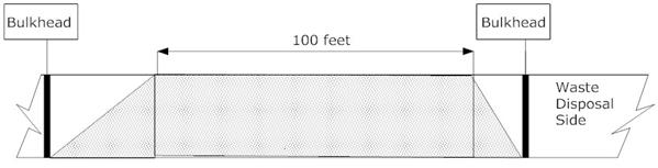
(a) Panel closure with 100 feet of ROM salt between two ventilation bulkheads

Appendix PA.tiff

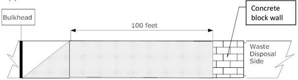
(b) Panel closure with 100 feet of ROM salt between a ventilation bulkhead and explosion wall

Figure PA- 16. Schematic Diagram of the ROMPCS

Material parameters and timings used to represent the ROMPCS are developed to account for the following physical processes and accepted rock mechanics principles:

1. Creep closure of the salt rock surrounding panel entries will cause consolidation of ROM salt emplaced in panel entries.

2. Eventually, the ROM salt comprising the closures will approach a condition similar to intact salt.

3. As ROM salt reaches higher fractional densities during consolidation, back stress will be imposed on the surrounding rock mass leading to eventual healing of the DRZ.

4. DRZ healing above and below the ROM salt panel closures will reduce DRZ porosity and permeability in those areas.

ROMPCS properties are based on three time periods (see Camphouse et al. 2012a, Camphouse 2013c, and Camphouse et al. 2013) to capture the temporal dependence of the physical processes listed above. Consequently, the ROMPCS is represented by three materials, with each material representing the ROMPCS for a portion of the 10,000-year regulatory period. Material PCS_T1 represents the ROMPCS for the first 100 years after facility closure. Material PCS_T2 models the ROMPCS from 100 to 200 years. Finally, material PCS_T3 represents the ROMPCS from years 200 to 10,000. For the first 200 years post-closure, the DRZ above and below the ROMPCS maintains the same properties as specified to the DRZ surrounding the disposal rooms (PA material DRZ_1). After 200 years, the DRZ above and below the ROMPCS is modeled as having healed, and is represented by material DRZ_PCS(see Figure PA-12 and Appendix MASS-2014, Section 4.1.3 ). Material DRZ_1 has the same properties in the CRA-2014 PA as were assigned to it in the CRA-2009 PABC. The permeability of material DRZ_PCS is modified slightly in the CRA-2014 PA as compared to the CRA-2009 PABC (see Appendix PA-2009, Section 4.2.8.3 for a discussion of material DRZ_PCS used in the CRA-2009 PABC). The healing of the DRZ region above and below the ROMPCS will not yield a higher permeability than that above the rooms. A relationship is implemented in the CRA-2014 PA to enforce that the permeability of material DRZ_PCS is never greater than the permeability of material DRZ_1. The constraint placed on the permeability for DRZ_PCS is that DRZ_PCS:PRMX ≤ DRZ_1:PRMX, and likewise in the y and z directions. If the sampled permeability for DRZ_PCS is greater than that obtained for DRZ_1, then DRZ_PCS retains the DRZ_1 permeability. The uncertainty distributions specified for the permeabilities of materials DRZ_1 and DRZ_PCS in the CRA-2014 PA are identical to those used in the CRA-2009 PABC.

As developed in Camphouse et al. (Camphouse et al. 2012b), permeability and porosity values are obtained through sampling for ROMPCS material PCS_T1. Porosity values are sampled for materials PCS_T2 and PCS_T3 and then used to calculate permeability values for these materials. The relationship used to calculate the permeability of material PCS_T2 is of the form

where k₂ is the calculated permeability for PCS_T2, f ₂ is the sampled PCS_T2 porosity value, and α is sampled from a normal distribution having a mean of 0, a standard deviation of 0.86,

and truncated at ±2 standard deviations. An analogous relationship is used for PCS_T3, and is of the form

Overlap in the porosity ranges for materials PCS_T1 and PCS_T2 potentially results in an increase in panel closure porosity during the transition from PCS_T1 to PCS_T2 at 100 years, a non-physical result. To prevent this possibility, the porosity for PCS_T2 is conditionally sampled so that PCS_T2:POROSITY ≤ PCS_T1:POROSITY for all vectors. For similar reasons, the porosity for material PCS_T3 is conditionally sampled so that PCS_T3:POROSITY ≤ PCS_T2:POROSITY. Similar constraints are placed on the calculated permeabilities for materials PCS_T2 and PCS_T3. The calculated permeability value for PCS_T2 is constrained such that PCS_T2:PRMX ≤ PCS_T1:PRMX. If the calculated permeability for PCS_T2 is greater than the sampled permeability for PCS_T1, then PCS_T2 retains the sampled PCS_T1 permeability. The same is true for the calculated permeabilities in the y and z directions. A similar constraint is placed on the calculated permeability for PCS_T3 in order to prevent non-physical instantaneous increases in panel closure permeability at 200 years. The constraint placed on the calculated permeability for PCS_T3 is that PCS_T3:PRMX ≤ PCS_T2:PRMX, and likewise in the x and y directions. If the calculated permeability for PCS_T3 is greater than the permeability for PCS_T2, then PCS_T3 retains the sampled PCS_T2 permeability. Uncertain parameters representing the ROMPCS are listed in Kicker and Herrick (Kicker and Herrick 2013), Table 4.

PA-4.2.9 Borehole Model

The major disruptive event in PA is the penetration of the repository by a drilling intrusion. The same numerical grid is used for undisturbed and borehole intrusion scenarios. In the undisturbed scenario (see Section PA-6.7.1), grid cells corresponding to the intrusion location have the material properties of the neighboring stratigraphic or excavated modeling unit. There is no designation in the borehole grid except for the reduced lateral dimensions of this particular column of grid cells.

In the scenarios simulating drilling disturbance, cells corresponding to the intrusion location start out with the same material properties as in the undisturbed scenario. At the time of intrusion, these cells are reassigned borehole material properties. The drilling intrusion is modeled by modifying the permeability of the grid blocks in Column 26 of Figure PA-12 (values listed in Table PA-7). Furthermore, the drilling intrusion is assumed to produce a borehole with a diameter of 12.25 in. (0.31115 m) (Vaughn 1996; Howard 1996), borehole fill is assumed to be incompressible, capillary effects are ignored, residual gas and brine saturations are set to zero, and porosity is set to 0.32 (see materials CONC_PLG, BH_OPEN, BH_SAND, and BH_CREEP in Table PA-3). When a borehole that penetrates pressurized brine in the Castile is simulated (i.e., an E1 intrusion), the permeability modifications indicated in Table PA-7 extend from the ground surface (i.e., Grid Cell 2155 in Figure PA-14) to the base of the pressurized brine (i.e., Grid Cell 2225 in Figure PA-14). When a borehole that does not penetrate pressurized brine in the Castile is under consideration (i.e., an E2 intrusion), the permeability modifications indicated in Table PA-7 stop at the floor of the intruded waste panel (i.e., Grid Cell 1419 in Figure PA-14).

PA-4.2.10 Castile Brine Reservoir

High-pressure Castile brine was encountered in several WIPP-area boreholes, including the WIPP-12 borehole within the controlled area and the U.S. Energy Research and Development Administration (ERDA)-6 borehole northeast of the site. Consequently, the conceptual model for the Castile includes the possibility that brine reservoirs underlie the repository. The E1 and E1E2 scenarios include borehole penetration of both the repository and a brine reservoir in the Castile.

Unless a borehole penetrates both the repository and a brine reservoir in the Castile, the Castile is conceptually unimportant to PA because of its expected low permeability. Two regions are specified in the disposal system geometry of the Castile horizon: the Castile (Rows 1 and 2 in Figure PA-12) and a reservoir (Row 1, Columns 23 to 45 in Figure PA-12). The Castile region has an extremely low permeability, which prevents it from participating in fluid flow processes.

Table PA- 7. Permeabilities for Drilling Intrusions Through the Repository

Time After Intrusion	Assigned Permeabilities
0-200 years	Concrete plugs are assumed to be emplaced at the Santa Rosa (i.e., a surface plug with a length of 15.76 m; corresponds to Grid Cells 2113, 2155 in Figure PA-14) and the Los Medaños Member of the Rustler (i.e., a plug at the top of the Salado with a length of 36 m; corresponds to Grid Cell 1644 in Figure PA-14). Concrete plugs are assumed to have a permeability log-uniformly sampled between 10^-19 m² to 10^-17m² (see material CONC_PLG in Kicker and Herrick (2013), Table 4). The open portions of the borehole are assumed to have a permeability of 1 ´ 10^-9 m².
200-1200 years	Concrete plugs are assumed to fail after 200 years (U.S. DOE 1995). An entire borehole is assigned a permeability typical of silty sand log-uniformly sampled between 10^-16.3 m² and 10^-11 m² (see parameter BHPRM and material BH_SAND in Kicker and Herrick 2013, Table 4).
> 1200 years	Permeability of borehole reduced by one order of magnitude in the Salado beneath the repository due to creep closure of borehole (Thompson et al. 1996) (i.e., k = 10 ^x /10, x = BHPRM, in Grid Cells 2225, 1576, 26, 94, 162, 230, 1135, 1142, 1149 of Figure PA-14) (see material BH_CREEP in Kicker and Herrick 2013, Table 4).

It is unknown whether a brine reservoir exists below the repository. As a result, the conceptual model for the brine reservoirs is somewhat different from those for known major properties of the natural barrier system, such as stratigraphy. The principal difference is that a reasonable treatment of the uncertainty of the existence of a brine reservoir requires assumptions about the spatial distribution of such reservoir and the probability of intersection (see Appendix MASS-2014, Section MASS.17.0 ). A range of probabilities for a borehole hitting a brine reservoir is used (see Section PA-3.6).

In addition to the stochastic uncertainty in the location and hence in the probability of intersecting reservoirs, there is also uncertainty in the properties of reservoirs. The manner in which brine reservoirs would behave if penetrated is captured by parameter ranges and is incorporated in the BRAGFLO calculations of disposal system performance. The conceptual model for the behavior of such a brine reservoir is discussed below. The properties specified for brine reservoirs are pressure, permeability, compressibility, and porosity, and are sampled from parameter ranges (see Table PA-17).

Where they exist, Castile brine reservoirs in the northern Delaware Basin are believed to be fractured systems, with high-angle fractures spaced widely enough that a borehole can penetrate through a volume of rock containing a brine reservoir without intersecting any fractures, and therefore not producing brine. Castile brine reservoirs occur in the upper portion of the Castile (Popielak et al. 1983). Appreciable volumes of brine have been produced from several reservoirs in the Delaware Basin, but there is little direct information on the areal extent of the reservoirs or the existence of the interconnection between them. Data from WIPP-12 and ERDA-6 indicate that fractures have a variety of apertures and permeabilities, and they deplete at different rates. Brine occurrences in the Castile behave as reservoirs; that is, they are bounded systems.

PA-4.2.11 Numerical Solution

Determining gas and brine flow in the vicinity of the repository requires solving the two nonlinear PDEs in Equation (PA.24), Equation (PA.25), Equation (PA.26), Equation (PA.27), Equation (PA.28), Equation (PA.29) and Equation (PA.30) on the computational domain in Figure PA-12, along with evaluating appropriate auxiliary conditions. The actual unknown functions in this solution are P _b and S _g , although the constraint conditions also give rise to values for P _g and S _b . As two dimensions in space and one dimension in time are in use, P _b , P _g , S _b , and S _g are functions of the form P _b (x, y, t), P _g (x, y, t), S _b (x, y, t), and S _g (x, y, t).

Solving Equation (PA.24), Equation (PA.25), Equation (PA.26), Equation (PA.27), Equation (PA.28), Equation (PA.29) and Equation (PA.30) requires both initial value and boundary value conditions for P _b and S _g . The initial value conditions for P _b and S _g are given in Section PA-4.2.2. As indicated there, the calculation starts at time t = −5 years, with a possible resetting of values at t = 0 years, which corresponds to final waste emplacement and sealing of the repository. The boundary conditions are such that no brine or gas moves across the exterior grid boundary (Table PA-8). This Neumann-type boundary condition is maintained for all time. Further, BRAGFLO allows the user to maintain a specified pressure and/or saturation at any grid

Table PA- 8. Boundary Value Conditions for P _g and P _b

Boundaries below (Row 1, y = 0 m) and above (Row 33, y = 1039 m) system for 0 £ x £ 46630 m (Columns 1-68) and -5 yr £ t. Below, j refers to the unit normal vector in the positive y direction.
× j = 0 Pa / m	No gas flow condition
× j = 0 Pa / m	No brine flow condition
Boundaries at left (Column 1, x = 0 m) and right (Column 68, x = 46630 m) of system for 0 £ y £ 1039 m (Rows 1-33) and -5 yr £ t. Below, i refers to the unit normal vector in the positive x direction.
× i = 0 Pa / m	No gas flow condition
× i = 0 Pa / m	No brine flow condition

block. This is not a boundary condition and is not required to close the problem. This feature is used to specify Dirichlet-type conditions at the surface grid blocks (Columns 1-68, Row 33, Figure PA-12) and at the far-field locations in the Culebra and Magenta (Columns 1 and 68, Row 26, and Columns 1 and 68, Row 28, Figure PA-12 ). These auxiliary conditions are summarized in Table PA-9.

Table PA- 9. Auxiliary Dirichlet Conditions for S _g and P _b

Surface Grid Blocks
= 0.08363	Columns 1-42, 44-68, Row 33, -5 yr £ t Saturation is not forced at the shaft cell on the surface because its saturation is reset to 1.0 at t = 0 yr.
= 1.01 ´ 10⁵ Pa	Columns 1-68, row 33, -5 yr £ t
Culebra and Magenta Far Field
= 9.14 ´ 10⁵ Pa	i = 1 and 68, j = 26, -5 yr £ t (Culebra)
= 9.47 ´ 10⁵ Pa	i = 1 and 68, j = 28, -5 yr £ t (Magenta)

A fully implicit finite-difference procedure is used to solve Equation (PA.24), Equation (PA.25), Equation (PA.26), Equation (PA.27), Equation (PA.28), Equation (PA.29) and Equation (PA.30). The associated discretization of the gas mass balance equation is given by

(PA.100)

where F represents the phase potentials given by

and

the subscripts are defined by

i = x-direction grid index

j = y-direction grid index

= x-direction grid block interface

= y-direction grid block interface

x _i = grid block center in the x-coordinate direction (m)

y _j = grid block center in the y-coordinate direction (m)

= grid block length in the x-coordinate direction (m)

= grid block length in the y-coordinate direction (m)

the superscripts are defined by

n = index in the time discretization, known solution time level

n+1 = index in the time discretization, unknown solution time level

and the interblock densities are defined by

The interface values of k _rg in Equation (PA.100) are evaluated using upstream weighted values (i.e., the relative permeabilities at each grid block interface are defined to be the relative permeabilities at the center of the adjacent grid block with the highest potential). Further, interface values for a r _gk _x / m _g and a r _gk _y / m _g are obtained by harmonic averaging of adjacent grid block values for these expressions. Currently all materials are isotropic, i.e. k _x = k _y = k _z .

The discretization of the brine mass balance equation is obtained by replacing the subscript for gas, g, by the subscript for brine, b. As a reminder, P _g and S _b are replaced in the numerical implementation with the substitutions indicated by Equation (PA.27) and Equation (PA.26), respectively. Wells are not used in the conceptual model for long-term Salado flow calculations, but they are used for DBR calculations. Thus, for long-term Salado flow calculations, the terms q _g and q _b are zero. For long-term Salado flow calculations, the wellbore is not treated by a well model, but rather is explicitly modeled within the grid as a distinct material region (i.e., Upper Borehole and Lower Borehole in Figure PA-12).

The resultant coupled system of nonlinear brine and gas mass balance equations is integrated in time using the Newton-Raphson method with upstream weighting of the relative permeabilities, as previously indicated. The primary unknowns at each computational cell center are brine pressure and gas saturation.

PA-4.2.12 Gas and Brine Flow across Specified Boundaries

The Darcy velocity vectors v _g (x, y, t) and v _b (x, y, t) for gas and brine flow (m³/m²/s = m/s) are defined by the expressions

(PA.101)

and

(PA.102)

Values for v _g and v _b are obtained and saved as the numerical solution of Equation (PA.24), Equation (PA.25), Equation (PA.26), Equation (PA.27), Equation (PA.28), Equation (PA.29) and Equation (PA.30) is carried out. Cumulative flows of gas, C _g (t, B), and brine, C _b (t, B), from time 0 to time t across an arbitrary boundary B in the domain of (Figure PA-12) is then given by

(PA.103)

for l = g, b, where a (x, y) is the geometry factor defined in Equation (PA.32), n(x, y) is an outward-pointing unit normal vector, and denotes a line integral. As an example, B could correspond to the boundary of the waste disposal regions in Figure PA-12. The integrals defining C _g (t, B) and C _b (t, B) are evaluated using the Darcy velocities defined by Equation (PA.101) and Equation (PA.102). Due to the dependence of gas volume on pressure, C _g (t, B) is typically calculated in moles or cubic meters at standard temperature and pressure, which requires an appropriate change of units for v _g in the calculation of C_l(t,B).

PA-4.2.13 Additional Information

Additional information on BRAGFLO and its use in the CRA-2014 PA can be found in the BRAGFLO user's manual (Camphouse 2013b), the BRAGFLO design document (Camphouse 2013a) and the analysis package for the Salado flow calculations in the CRA-2014 PA (Camphouse 2013c).

PA-4.3 Radionuclide Transport in the Salado: NUTS

The NUTS code is used to model radionuclide transport in the Salado. NUTS models radionuclide transport within all regions for which BRAGFLO computes brine and gas flow, and for each realization uses as input the corresponding BRAGFLO velocity field, pressures, porosities, saturations, and other model parameters, including, for example, the geometrical grid, residual saturation, material map, and compressibility. Of the radionuclides that are transported vertically due to an intrusion or up the shaft, without reaching the surface as a DBR, it is assumed that the lateral radionuclide transport is in the most transmissive unit, the Culebra. Therefore, the radionuclide transport through the Dewey Lake to the accessible environment and to the land surface due to long-term flow are set to zero.

The PA uses NUTS in two different modes. First, the code is used in a computationally fast screening mode to identify those BRAGFLO realizations for which it is unnecessary to do full transport calculations because the amount of contaminated brine that reaches the Culebra or the LWB within the Salado is insufficient to significantly contribute to the total integrated release of radionuclides from the disposal system. For the remaining realizations, which have the possibility of consequential release, a more computationally intensive calculation of each radionuclide's full transport is performed (see Section PA-6.7.2).

This section describes the model used to compute radionuclide transport in the Salado for E0, E1, and E2 scenarios (defined in Section PA-2.3.2). The model for transport in the E1E2 scenario, which is computed using the PANEL code, is described in Section PA-4.4.

NUTS models radionuclide transport by advection (see Appendix MASS-2014, Section MASS-12.5 ). NUTS disregards sorptive and other retarding effects throughout the entire flow region. Physically, some degree of retardation must occur at locations within the repository and the geologic media; it is therefore conservative to ignore retardation processes. NUTS also ignores reaction-rate aspects of dissolution and colloid formation processes, and mobilization is assumed to occur instantaneously. Neither molecular nor mechanical dispersion is modeled in NUTS. These processes are assumed to be insignificant compared to advection, as discussed further in Appendix MASS-2014, Section MASS-12.5.

Colloidal actinides are subject to retardation by chemical interaction between colloids and solid surfaces and by clogging of small pore throats (i.e., by sieving). There will be some interaction of colloids with solid surfaces in the anhydrite interbeds. Given the low permeability of intact interbeds, it is likely that pore apertures will be small and some sieving will occur. However, colloidal particles, if not retarded, are transported slightly more rapidly than the average velocity of the bulk liquid flow. Because the effects on transport of slightly increased average pore velocity and retarded interactions with solid surfaces and sieving offset one another, the DOE assumes residual effects of these opposing processes will be either small or beneficial, and does not incorporate them when modeling actinide transport in the Salado interbeds.

If brine in the repository moves into interbeds, it is likely that mineral precipitation reactions will occur. Precipitated minerals may contain actinides as trace constituents. Furthermore, colloidal-sized precipitates will behave like mineral-fragment colloids, which are destabilized by brines, quickly agglomerating and settling by gravity. The beneficial effects of precipitation and coprecipitation are neglected in PA.

Fractures, channeling, and viscous fingering may also impact transport in Salado interbeds, which contain natural fractures. Because of the low permeability of unfractured anhydrite, most fluid flow in interbeds will occur in fractures. Even though some properties of naturally fractured interbeds are characterized by in situ tests, uncertainty exists in the characteristics of the fracture network that may be created with high gas pressure in the repository. The PA modeling system accounts for the possible effects on porosity and permeability of fracturing by using a fracturing model (see Section PA-4.2.4). The processes and effects associated with fracture dilation or fracture propagation not already captured by the PA fracture model are negligible (see the CCA, Appendix MASS, Section MASS.13.3 and Appendix MASS, Attachment 13.2). Of those processes not already incorporated, channeling has the greatest potential effect.

Channeling is the movement of fluid through the larger-aperture sections of a fracture network with locally high permeabilities. It could locally enhance actinide transport. However, it is assumed that the effects of channeled flow in existing or altered fractures will be negligible for the length and time scales associated with the disposal system. The DOE believes this assumption is reasonable because processes are likely to occur that limit the effectiveness of channels or the dispersion of actinides in them. First, if gas is present in the fracture network, it will be present as a nonwetting phase and will occupy theportions of the fracture network with relatively large apertures, where the highest local permeabilities will exist. The presence of gas thus removes the most rapid transport pathways from the contaminated brine and decreases the impact of channeling. Second, brine penetrating the Salado from the repository is likely to be completely miscible with in situ brine. Because of miscibility, diffusion or other local mixing processes will probably broaden fingers (reduce concentration gradients) until the propagating fingers are indistinguishable from the advancing front.

Gas will likely penetrate the liquid-saturated interbeds as a fingered front, rather than a uniform front. Fingers form when there is a difference in viscosity between the invading fluid (gas) and the resident fluid (liquid brine), and because of channeling effects. This process does not affect actinide transport, however, because actinides of interest are transported only in the liquid phase, which will not displace gas in the relatively high-permeability regions due to capillary effects.

PA-4.3.1 Mathematical Description

The following system of PDEs is used to model radionuclide transport in the Salado:

- Ñ × (PA.104)

(PA.105)

for l = 1, 2, …, n _R , where

= Darcy velocity vector (m³/m²/s = m/s) for brine (supplied by BRAGFLO from solution of Equation (PA.102))

C bl = concentration (kg/m³) of radionuclide l in brine

C sl = concentration (kg/m³) of radionuclide l in solid phase (i.e., not in brine), with concentration defined with respect to total (i.e., bulk) formation volume (only used in repository; see Figure PA-12)

S l = linkage term (kg/m³/s) due to dissolution/precipitation between radionuclide l in brine and in solid phase (see Equation (PA.106))

f = porosity (supplied by BRAGFLO from solution of Equation (PA.24), Equation (PA.25), Equation (PA.26), Equation (PA.27), Equation (PA.28), Equation (PA.29) and Equation (PA.30))

S b = brine saturation (supplied by BRAGFLO from solution of Equation (PA.24), Equation (PA.25), Equation (PA.26), Equation (PA.27), Equation (PA.28), Equation (PA.29) and Equation (PA.30))

l l = decay constant (s^-1) for radionuclide l

P(l) = {p: radionuclide p is a parent of radionuclide l}

n _R = number of radionuclides,

and a is the dimension-dependent geometry factor in Equation (PA.32). PA uses a two-dimensional representation for fluid flow and radionuclide transport in the vicinity of the repository, with a defined by the element depths in Figure PA-12. Although omitted for brevity, the terms a, v _b , C _bl , C _sl , S _l , S _b , and f are functions a (x, y), v _b (x, y, t), C _bl (x, y, t), C _sl (x, y, t), S _l (x, y, t), S _b (x, y, t), and f (x, y, t) of time t and the spatial variables x and y. Equation (PA.104) and Equation (PA.105) are defined and solved on the same computational grid (Figure PA-12) used by BRAGFLO for the solution of Equation (PA.24), Equation (PA.25), Equation (PA.26), Equation (PA.27), Equation (PA.28), Equation (PA.29) and Equation (PA.30).

Radionuclides are assumed to be present in both brine (Equation (PA.104)) and in an immobile solid phase (Equation (PA.105)), although radionuclide transport takes place only by brine flow (Equation (PA.104)). Maximum radionuclide concentrations are calculated for elements dissolved in Salado and Castile brines for oxidation states III, IV, and V. Maximum concentrations are dependent on the dissolved solubility (mols per liter mol/L) for each brine type and oxidation state, as well as the uncertainty associated with the dissolved solubility. Dissolved solubilities and their uncertainties are developed in Brush and Domski (Brush and Domski 2013b and Brush and Domski 2013c), and are listed in Kicker and Herrick (Kicker and Herrick 2013), Table 27, Table A-8 , and Table A-9. Only the maximum concentration corresponding to the minimum brine volume of 17,400 m³ is used in Salado transport calculations due to the computational expense associated with NUTS. This approach is conservative as it maximizes the concentration of actinides that are potentially transported across the LWB.

The maximum radionuclide concentration is assumed to equilibrate instantly for each element (Am, Pu, U, Th). Then each individual radionuclide equilibrates between the brine and solid phases based on the maximum concentration of the radionuclide and the mole fractions of other isotopes included in the calculation. The linkage between the brine and solid phases in Equation (PA.104) and Equation (PA.105) is accomplished by the term S _l , where

(PA.106)

where

= maximum concentration (kg/m³) of element El(l) in oxidation state Ox(l) in brine type Br(t), where El(l) denotes the element of which radionuclide l is an isotope, Ox(l) denotes the oxidation state in which element El(l) is present, and Br(t) denotes the type of brine present in the repository at time t.

= concentration (kg/m3) of element El(l) in brine (p = b) or solid (p = s), which is equal to the sum of concentrations of radionuclides that are isotopes of same element as radionuclide l, where k Î El(l) only if k is an isotope of element El(l):

(PA.107)

= difference (kg/m³) between maximum concentration of element El(l) in brine and existing concentration of element El(l) in brine

(PA.108)

MF pl = mole fraction of radionuclide l in phase p, where p = b (brine) or
p = s (solid)

(PA.109)

CM l = conversion factor (mol/kg) from kilograms to moles for radionuclide l

= Dirac delta function (s^- ¹) ( d ( t - t) = 0 if t ¹ t and )

The terms S _l , S _b , C _p,El(l) , MF _pl , and f are functions of time t and the spatial variables x and y, although the dependencies are omitted for brevity. The Dirac delta function, d( t - t), appears in Equation (PA.106) to indicate that the adjustments to concentration are implemented instantaneously within the numerical solution of Equation (PA.104) and Equation (PA.105) whenever a concentration imbalance is observed.

The velocity vector v _b in Equation (PA.104) and Equation (PA.105) is defined in Equation (PA.102) and is obtained from the numerical solution of Equation (PA.24), Equation (PA.25), Equation (PA.26), Equation (PA.27), Equation (PA.28), Equation (PA.29) and Equation (PA.30). If B denotes an arbitrary boundary (e.g., the LWB) in the domain of Equation (PA.104) and Equation (PA.105) (as shown in Figure PA-12), the cumulative transport of C _l (t, B) of radionuclide l from time 0 to time t across B is given by

(PA.110)

where n (x, y) is an outward-pointing unit normal vector and denotes a line integral over B.

Equation (PA.104) and Equation (PA.105) models advective radionuclide transport due to the velocity vector v _b .

PA-4.3.2 Radionuclides Transported

Since the solution of Equation (PA.104) and Equation (PA.105) for many radionuclides and decay chains is computationally very expensive, the number of radionuclides for direct inclusion in the analysis is initially reduced using the algorithm shown in Figure PA-17. The number of radionuclides included in the transport calculations is then further reduced by combining those with similar decay and transport properties. The CRA-2014 PA uses the same reduction algorithm as the CCA PA (see the CCA, Appendix WCA); the algorithm was found to be acceptable in the CCA review (U.S. EPA 1998a, Section 4.6.1.1 ).

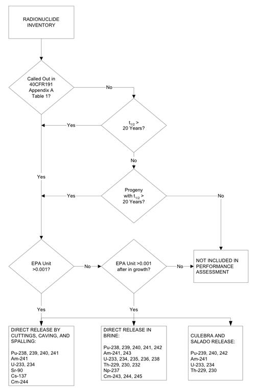
Figure PA- 17. Selecting Radionuclides for the Release Pathways Conceptualized by PA

Using Figure PA-17, the number of radionuclides initially included in the decay calculations is 29. These radionuclides are the same as those in the CRA-2009 PABC, and belong to the following decay chains:

(PA.111)

(PA.112)

(PA.113)

(PA.114)

Radionuclides considered in the decay calculations that do not belong to one of the decay chains listed above are ¹⁴⁷Pm, ¹³⁷Cs, and ⁹⁰Sr. In addition, some intermediates with extremely short half-lives, such as ²⁴⁰U, were omitted from the decay chains.

Further simplification of the decay chains is possible based on the total inventories. Releases of radionuclides whose inventories total less than one EPA unit are essentially insignificant, as any release that transports essentially all of a given species outside the LWB will be dominated by the releases of other species with much larger inventories. In addition, ¹³⁷Cs and ⁹⁰Sr can be omitted because their concentrations drop to below 1 EPA unit within 150 years, which makes it improbable that a significant release of these radionuclides will occur.

After the reduction of radionuclides outlined in Figure PA-17 and the paragraph above, the following 10 radionuclides remained from the decay chains shown:

(PA.115)

(PA.116)

(PA.117)

(PA.118)

²³⁸Pu does not significantly affect transport calculations because of its short half-life (87.8 years). The remaining nine radionuclides were then further reduced by combining those with similar decay and transport properties. In particular, ²³⁴U, ²³⁰Th, and ²³⁹Pu were used as surrogates for the groups {²³⁴U, ²³³U}, {²³⁰Th, ²²⁹Th}, and {²⁴²Pu, ²⁴⁰Pu, ²³⁹Pu}, with the initial inventories of ²³⁴U, ²³⁰Th, and ²³⁹Pu being increased to account for the additional radionuclide(s) in each group.

In increasing the initial inventories, the individual radionuclides were combined (or "lumped" together) on either a mole or curie basis (i.e., moles added and then converted back to curies, or curies added directly (see Kicker and Zeitler 2013b)). In each case, the method that maximized the combined inventory was used; thus, ²³³U was added to ²³⁴U, ²⁴⁰Pu to ²³⁹Pu, and ²²⁹Th to ²³⁰Th by curies, while ²⁴²Pu was added to ²³⁹Pu by moles. In addition, ²⁴¹Pu was added to ²⁴¹Am by moles because ²⁴¹Pu has a half-life of 14 years and will quickly decay to ²⁴¹Am. The outcome of this process was the following set of five radionuclides in three simplified decay chains:

( PA.119)

which were then used with Equation (PA.104) and Equation (PA.105) for transport in the vicinity of the repository. The development of these "lumped" radionuclide inventories is done in Kicker and Zeitler (Kicker and Zeitler 2013b), and the results are listed in Kicker and Herrick (Kicker and Herrick 2013), Table 29. These "lumped" radionuclides closely approximate the activity of the total normalized waste inventory (Kim 2013b).

PA-4.3.3 NUTS Tracer Calculations

All BRAGFLO realizations are first evaluated using NUTS in a screening mode to identify those realizations for which a significant release of radionuclides to the LWB cannot occur. The screening simulations consider an infinitely soluble, nondecaying, nondispersive, and nonsorbing species as a tracer element. The tracer is given a unit concentration in all waste disposal areas of 1 kg/m³. If the amount of tracer that reaches the selected boundaries (the top of the Salado and the LWB within the Salado) does not exceed a cumulative mass of 10^-7 kg within 10,000 years, it is assumed there is no consequential release to these boundaries. If the cumulative mass outside the boundaries within 10,000 years exceeds 10^-7 kg, a complete transport analysis is conducted. The value of 10^- ⁷ kg is selected because, regardless of the isotopic composition of the release, it corresponds to a normalized release less than 10^-6 EPA units, the smallest release displayed in CCDF construction (Stockman 1996). The largest normalized release would be 9.98 × 10^-7 EPA units, corresponding to 10^- ⁷ kg of ²⁴¹Am if the release was entirely ²⁴¹Am.

PA-4.3.4 NUTS Transport Calculations

For BRAGFLO realizations with greater than 10^- ⁷ kg reaching the boundaries in the tracer calculations, NUTS models the transport of five different radionuclide species (²⁴¹Am, ²³⁹Pu, ²³⁸Pu, ²³⁴U, and ²³⁰Th). These radionuclides represent a larger number of radionuclides; as discussed in Section PA-4.3.2, radionuclides were grouped together based on similarities, such as isotopes of the same element and those with similar half-lives, to simplify the calculations. For transport purposes, solubilities are lumped to represent both dissolved and colloidal forms. These groupings simplify and expedite calculations.

PA-4.3.5 Numerical Solution

Equation (PA.104) and Equation (PA.105) are numerically solved by the NUTS program (WIPP Performance Assessment 1997a) on the same computational grid (Figure PA-12) used by BRAGFLO for the solution of Equation (PA.24), Equation (PA.25), Equation (PA.26), Equation (PA.27), Equation (PA.28), Equation (PA.29), and Equation (PA.30). In the solution procedure, Equation (PA.104) and Equation (PA.105) are numerically solved with S _l = 0 for each time step, with the instantaneous updating of concentrations indicated in Equation (PA.106) and the appropriate modification to C _sl in Equation (PA.105) taking place after the time step. The solution is carried out for the five radionuclides indicated in Equation (PA.119).

The initial value and boundary value conditions used with Equation (PA.104) and Equation (PA.105) are given in Table PA-10. At time t = 0 (corresponding to the year 2033), the total inventory of each radionuclide is assumed to be in brine; the solubility constraints associated with Equation (PA.106) then immediately adjust the values for C _bl (x, y, t) and C _sl (x, y, t) for consistency with the constraints imposed by S _T (Br, Ox, El) and available radionuclide inventory.

The n _R PDEs in Equation (PA.104) and Equation (PA.105) are discretized in two dimensions and then developed into a linear system of algebraic equations for numerical implementation. The following conventions are used in the representation of each discretized equation:

· The subscript b is dropped from C _bl, so that the unknown function is represented by C _l.

· A superscript n denotes time t _n, with the assumption that the solution C _l is known at time t _n and is to be propagated to time t _n+1.

· The grid indices are i in the x-direction and j in the y-direction, and are the same as the BRAGFLO grid indices.

Table PA- 10. Initial and Boundary Conditions for C _bl(x, y, t) and C _sl(x, y, t)

Initial Conditions for C _bl(x, y, t) and C _sl(x, y, t)

= if (x, y) is a point in the repository (i.e., areas Waste Panel, South RoR and North RoR, in Figure PA-12), where A_l (0) is the amount (kg) of radionuclide l present at time t = 0 and V_b (0) is the amount (m³) of brine in repository at time t = 0 (from solution of Equation (PA.24), Equation (PA.25), Equation (PA.26), Equation (PA.27), Equation (PA.28), Equation (PA.29) and Equation (PA.30) with BRAGFLO) for all (x, y).

= 0 otherwise.

= 0 if (x, y) is a point in the repository.

Boundary Conditions for C _bl(x, y, t)

= , where B is any subset of the outer boundary of the computational grid in Figure PA-12, is the flux (kg/s) at time t of radionuclide l across B, v _b (x, y, t) is the Darcy velocity (m³/m²/s) of brine at (x, y) on B and is obtained from the solution of Equation (PA.24) Equation (PA.25), Equation (PA.26), Equation (PA.27), Equation (PA.28), Equation (PA.29), and Equation (PA.30) by BRAGFLO, n (x, y) denotes an outward-pointing unit normal vector, and denotes a line integral along B.

· Fractional indices refer to quantities evaluated at grid block interfaces.

· Each time step by NUTS is equal to 20 BRAGFLO time steps because BRAGFLO stores results (here, v _b, f , and S _b) every 20 time steps.

The following finite-difference discretization is used for the l ^th equation in each grid block (i, j):

(PA.120)

where q _b is the grid block interfacial brine flow rate (m³/s) and V _R is the grid block volume (m³). The quantity q _b is based on and a in Equation (PA.104) and Equation (PA.105), and the quantity V _R is based on grid block dimensions (Figure PA-12) and a.

The interfacial values of concentration in Equation (PA.120) are discretized using the one-point upstream weighting method (Aziz and Settari 1979), which results in

(PA.121)

where w derives from the upstream weighting for flow between adjacent grid blocks and is defined by

By collecting similar terms, Equation (PA.121) can be represented by the linear equation

(PA.122)

where

Given the form of Equation (PA.122), the solution of Equation (PA.104) and Equation (PA.105) has now been reduced to the solution of n _R ´ n _G linear algebraic equations in n _R ´ n _G unknowns, where n _R is the number of equations for each grid block (i.e., the number of radionuclides) and n _G is the number of grid blocks into which the spatial domain is discretized (Figure PA-12).

The system of PDEs in Equation (PA.104) and Equation (PA.105) is strongly coupled because of the contribution from parental decay to the equation governing the immediate daughter. Consequently, a sequential method is used to solve for the radionuclide concentrations by starting at the top of a decay chain and working down from parent to daughter. This implies that when solving Equation (PA.122) for the l ^th isotope concentration, all parent concentrations occurring in the right-hand-side term R are known. The system of equations is then linear in the concentrations of the l ^th isotope. As a result, solving Equation (PA.104) and Equation (PA.105) is reduced from the solution of one algebraic equation at each time step with n _R ´ n _G unknowns to the solution of n _R algebraic equations each with n _G unknowns at each time step, which can result in a significant computational savings.

The matrix resulting from one-point upstream weighting has the following structural form for a 3 ´ 3 system of grid blocks, and a similar structure for a larger number of grid blocks:

	1	2	3	4	5	6	7	8	9
1	X	X	0	X
2	X	X	X	0	X
3	0	X	X	0	0	X
4	X	0	0	X	X	0	X
5		X	0	X	X	X	0	X
6			X	0	X	X	0	0	X
7				X	0	0	X	X	0
8					X	0	X	X	X
9						X	0	X	X

where X designates possible nonzero matrix entries, and 0 designates zero entries within the banded structure. All entries outside of the banded structure are zero. Because of this structure, a banded direct elimination solver (Aziz and Settari 1979, Section 8.2.1 ) is used to solve the linear system for each radionuclide. The bandwidth is minimized by first indexing equations in the coordinate direction with the minimum number of grid blocks. The coefficient matrix is stored in this banded structure, and all infill coefficients calculated during the elimination procedure are contained within the band structure. Therefore, for the matrix system in two dimensions, a pentadiagonal matrix of dimension I _BW ´ n _G is inverted instead of a full n _G ´ n _G matrix, where I _BW is the bandwidth.

The numerical implementation of Equation (PA.105) enters the solution process through updates to the radionuclide concentrations in Equation (PA.121) between each time step, as indicated in Equation (PA.106). The numerical solution of Equation (PA.104) and Equation (PA.105) also generates the concentrations required to numerically evaluate the integral that defines C _l (t, B) in Equation (PA.110).

PA-4.3.6 Additional Information

Additional information on NUTS and its use in WIPP PA can be found in the NUTS users manual (WIPP Performance Assessment 1997a) and in the analysis package of Salado transport calculations for the CRA-2014 PA (Kim 2013a). Furthermore, additional information on dissolved and colloidal actinides is given in Appendix SOTERM-2014, Section SOTERM-5.0.

PA-4.4 Radionuclide Transport in the Salado: PANEL

This section describes the model used to compute radionuclide transport in the Salado for the E1E2 scenario. The model for transport in E0, E1, and E2 scenarios is described in Section PA-4.3.

PA-4.4.1 Mathematical Description

A relatively simple mixed-cell model is used for radionuclide transport in the vicinity of the repository after an E1E2 intrusion, when connecting flow between two drilling intrusions into the same waste panel is assumed to take place. With this model, the amount of radionuclide l contained in a waste panel is represented by

(PA.123)

where

= amount (mol) of radionuclide l in waste panel at time t

= concentration (mol/m³) of radionuclide l in brine in waste panel at time t (Equation (PA.124) and Equation (PA.125))

= rate (m³/s) at which brine flows out of the repository at time t (supplied by BRAGFLO from solution of Equation (PA.102))

and l _l and P(l) are defined in conjunction with Equation (PA.104) and Equation (PA.105).

The brine concentration C _bl in Equation (PA.123) is defined by

(PA.124)

(PA.125)

where

= mole fraction of radionuclide l in waste panel at time t

= (PA.126)

= volume (m³) of brine in waste panel at time t (supplied by BRAGFLO from solution of Equation (PA.24), Equation (PA.25), Equation (PA.26), Equation (PA.27), Equation (PA.28), Equation (PA.29), and Equation (PA.30))

and S _T [Br, Ox, El] is the maximum concentration expressed in units of mol/L. Quantity C _bl (t) is defined to be the maximum concentration S_T if there is sufficient radionuclide inventory in the waste panel to generate this concentration (Equation (PA.124)); otherwise, C _bl (t) is defined by the concentration that results when all the relevant element in the waste panel is placed in solution (Equation (PA.125)). The dissolved and colloidal actinides equilibrate instantly for each element.

Given r _b and C _bl , evaluation of the integral

(PA.127)

provides the cumulative release R _l (t) of radionuclide l from the waste panel through time t.

PA-4.4.2 Numerical Solution

Equation (PA.123) is numerically evaluated by the PANEL model (WIPP Performance Assessment 1998b) using a discretization based on time steps of 50 years or less. Specifically, Equation (PA.123) is evaluated with the approximation

(PA.128)

where

= gain in radionuclide l due to the decay of precursor radionuclides between t n

and t n +1 (see Equation (PA.129)), = .

As the solution progresses, values for C _bl (t _n ) are updated in consistency with Equation (PA.124) and Equation (PA.125), and the products r _b (t _n )C _bl (t _n ) are accumulated to provide an approximation to R _l in Equation (PA.127).

The term G _l (t _n , t _n+1 ) in Equation (PA.128) is evaluated with the Bateman equations (Bateman 1910), with PANEL programmed to handle decay chains of up to five (four decay daughters for a given radionuclide). As a single example, if radionuclide l is the third radionuclide in a decay chain (i.e., l = 3) and the two preceding radionuclides in the decay chain are designated by l = 1 and l = 2, then

(PA.129)

in Equation (PA.128).

PA-4.4.3 Implementation in PA

The preceding model is used in two ways in PA. First, Equation (PA.127) estimates releases to the Culebra associated with E1E2 intrusion scenarios (see Section PA-6.7.3). Second, radionuclide concentrations are calculated that correspond to multiples of the minimum brine volume (17,400 m³) necessary for a DBR. Concentrations corresponding to the minimum brine volume comprise the S _l term indicated in Equation (PA.106) used in the NUTS calculations for Salado transport. Concentrations calculated over the range of brine volumes are used to determine releases when a volume of brine is released to the ground surface during a drilling intrusion.

For E1E2 intrusions, the initial amount A _l of radionuclide l is the inventory of the decayed isotope at the time of the E1 intrusion. PANEL calculates the inventory of each of the 29 radioisotopes throughout the regulatory period. The initial concentration C _bl of radionuclide l is computed by Equation (PA.123), Equation (PA.124), and Equation (PA.125). For the DBR calculations, the initial amount A _l of radionuclide l is the inventory of the isotope at the time of repository closure.

PA-4.4.4 Additional Information

Additional information on PANEL and its use in the CRA-2014 PA calculations can be found in the PANEL user's manual (WIPP Performance Assessment 2003a), the analysis package for PANEL calculations (Kim 2013b), and the analysis package for Salado transport calculations in the CRA-2014 PA (Kim 2013a).

PA-4.5 Cuttings and Cavings to Surface: CUTTINGS_S

Cuttings are waste solids contained in the cylindrical volume created by the cutting action of the drill bit passing through the waste, while cavings are additional waste solids eroded from the borehole by the upward-flowing drilling fluid within the borehole. The releases associated with these processes are computed within the CUTTINGS_S code (WIPP Performance Assessment 2003b). The mathematical representations used for cuttings and cavings are described in this section.

PA-4.5.1 Cuttings

The uncompacted volume of cuttings removed and transported to the surface in the drilling fluid, V _cut , is given by

(PA.130)

where A is the drill bit area (m²), H _i is the initial (or uncompacted) repository height (3.96 m) (see parameter BLOWOUT:HREPO in Kicker and Herrick 2013, Table 5), and D is the drill-bit diameter (0.31115 m) (see parameter BOREHOLE:DIAMMOD in Kicker and Herrick 2013, Table 5). For drilling intrusions through RH-TRU waste, H _i = 0.509 m is used (see parameter REFCON:HRH in Kicker and Herrick 2013, Table 37).

PA-4.5.2 Cavings

The cavings component of the direct surface release is caused by the shearing action of the drilling fluid on the waste as it flows up the borehole annulus. Like the cuttings release, the cavings release is assumed to be independent of the conditions that exist in the repository during a drilling intrusion.

The final diameter of the borehole depends on the diameter of the drillbit and on the extent to which the actual borehole diameter exceeds the drill-bit diameter. Although a number of factors affect erosion within a borehole (Chambre Syndicale de la Recherche et de la Production du Petrole et du Gaz Naturel 1982), the most important is the fluid shear stress on the borehole wall (i.e., the shearing force per unit area, N/m²) resulting from circulating drilling fluids (Darley 1969, Walker and Holman 1971). As a result, PA estimates cavings removal with a model based on the effect of shear stress on the borehole diameter. In particular, the borehole diameter is assumed to grow until the shear stress on the borehole wall is equal to the shear strength of the waste, which is the limit below which waste erosion ceases.

The final eroded diameter D _f (m) of the borehole through the waste determines the total volume V (m³) of uncompacted waste removed to the surface by circulating drilling fluid. Specifically,

(PA.131)

where V _cav is the volume (m³) of waste removed as cavings.

Most borehole erosion is believed to occur in the vicinity of the drill collar (Figure PA-18) because of decreased flow area and consequent increased mud velocity (Rechard, Iuzzolino, and Sandha 1990, Letters 1a and 1b, App. A). An important determinant of the extent of this erosion is whether the flow of the drilling fluid in the vicinity of the collar is laminar or turbulent. PA uses Reynolds numbers to distinguish between the occurrence of laminar flow and turbulent flow. The Reynolds number is the ratio between inertial and viscous (or shear) forces in a fluid, and can be expressed as (Fox and McDonald 1985)

(PA.132)

where Re is the Reynolds number (dimensionless), r _f is the fluid density (kg/m³), D _e is the equivalent diameter (m), is the fluid speed (m s^- ¹), and h is the fluid viscosity (kg m^- ¹ s^- ¹).

Typically, r _f , v, and h are averages over a control volume with an equivalent diameter of D _e , where r _f = 1.21 ´ 10³ kg/m³ (see parameter DRILLMUD:DNSFLUID in Kicker and Herrick 2013, Table 5), v = 0.7089 m s^- ¹ (based on 40 gal/min/in of drill diameter) (Berglund 1992), and D _e = 2 (R - R _i ), as shown in Figure PA-18. The diameter of the drill collar (i.e., 2R _i in Figure PA-18) is 8.0 in = 0.2032 m (Kicker 2013). The determination of h is discussed below. PA assumes that Reynolds numbers less than 2100 are associated with laminar flow, while Reynolds numbers greater than 2100 are associated with turbulent flow (Walker 1976).

Figure PA- 18. Detail of Rotary Drill String Adjacent to Drill Bit

Drilling fluids are modeled as non-Newtonian, which means that the viscosity h is a function of the shear rate within the fluid (i.e., the rate at which the fluid velocity changes normal to the flow direction, m/s/m). PA uses a model proposed by Oldroyd (1958) to estimate the viscosity of drilling fluids. As discussed in the Drilling Mud and Cement Slurry Rheology Manual (Chambre Syndicale de la Recherche et de la Production du Petrole et du Gaz Naturel 1982), the Oldroyd model leads to the following expression for the Reynolds number associated with the helical flow of a drilling fluid within an annulus:

(PA.133)

where r _f , D _e , and v are defined as in Equation (PA.132), and h _¥ is the asymptotic value for the derivative of the shear stress ( t , kg m^- ¹ s^- ²) with respect to the shear rate (G, s^- ¹) obtained as the shear rate increases (i.e., as ). PA uses Equation (PA.133) to determine whether drilling fluids in the area of the drill collar are undergoing laminar or turbulent flow.

The Oldroyd model assumes that the shear stress t is related to the shear rate G through the relationship

(PA.134)

where h ₀ is the asymptotic value of the viscosity (kg m^- ¹ s^- ¹) that results as the shear rate G approaches zero, and s ₁ and s ₂ are constants (s²). The expression leads to

(PA.135)

PA uses values of h ₀ = 1.834 ´ 10^- ² kg m^- ¹ s^- ¹, s ₁ = 1.082 ´ 10^- ⁶ s², and s ₂ = 5.410 ´ 10^- ⁷ s² (Berglund 1996), from which viscosity in the limit of infinite shear rate is found to be h _¥ = 9.17 ´ 10^- ³ kg m^- ¹ s^- ¹. The quantity h _¥ is comparable to the plastic viscosity of the fluid (Chambre Syndicale de la Recherche et de la Production du Petrole et du Gaz Naturel 1982).

As previously indicated, different models are used to determine the eroded diameter D _f of a borehole depending on whether flow in the vicinity of the drill collar is laminar or turbulent. The model for borehole erosion in the presence of laminar flow is described next, and then the model for borehole erosion in the presence of turbulent flow is described.

PA-4.5.2.1 Laminar Flow Model

As shown by Savins and Wallick (1966), the shear stresses associated with the laminar helical flow of a non-Newtonian fluid, as a function of the normalized radius, r, can be expressed as

(PA.136)

for R _i /R £ r £ 1, where R _i and R are the inner and outer radii within which the flow occurs, as indicated in Figure PA-18; t (R, r ) is the shear stress (kg m^- ¹ s^- ²) at a radial distance D R beyond the inner boundary (i.e., at r = (R _i + D R)/R); and the variables C, J, and l depend on R and satisfy conditions Equation (PA.138), Equation (PA.139) and Equation (PA.140). The shear stress at the outer radius R is given by

(PA.137)

As previously indicated, the borehole radius R is assumed to increase as a result of erosional processes until a value of R is reached at which t ( R, 1) is equal to the shear strength of the waste. In PA, the shear strength of the waste is represented by the uncertain parameter BOREHOLE:TAUFAIL that has a minimum of 2.22 Pa and a maximum of 77.0 Pa (see Kicker and Herrick 2013, Table 4). Computationally, determining the eroded borehole diameter R associated with a particular value of the waste shear strength requires repeated evaluation of t ( R, 1), as indicated in Equation (PA.137), until a value of R is determined for which t ( R, 1) equals the shear strength.

The quantities C, J, and l must satisfy the following three conditions (Savins and Wallick 1966) for Equation (PA.137) to be valid:

(PA.138)

(PA.139)

(PA.140)

where h , the drilling fluid viscosity (kg m^- ¹ s^- ¹), is a function of R and r ; D W is the drill string angular velocity (rad s^- ¹); and Q is the drilling fluid flow rate (m³ s^- ¹).

The viscosity h in Equation (PA.138), Equation (PA.139) and Equation (PA.140) is introduced into the analysis by assuming that the drilling fluid follows the Oldroyd model for shear stress in Equation (PA.134). By definition of the viscosity h ,

t = h G (PA.141)

and from Equation (PA.134)

(PA.142)

thus the expression in Equation (PA.136) can be reformulated as

(PA.143)

As discussed by Savins and Wallick (1966) and Berglund (1992), the expressions in Equation (PA.138), (Equation (PA.139) and Equation (PA.140) and Equation (PA.142) can be numerically evaluated to obtain C, J, and l for use in Equation (PA.136) and Equation (PA.137). In PA, the drill string angular velocity D W is treated as an uncertain parameter (see DOMEGA in Table PA-17), and

(PA.144)

where v = 0.7089 m s^- ¹ as used in Equation (PA.132), and h ₀, s ₁ , and s ₂ are defined as in Equation (PA.134) and Equation (PA.135).

PA-4.5.2.2 Turbulent Flow Model

The model for borehole erosion in the presence of turbulent flow is now described. Unlike the theoretically derived relationship for erosion in the presence of laminar flow, the model for borehole erosion in the presence of turbulent flow is empirical. In particular, pressure loss for axial flow in an annulus under turbulent flow conditions can be approximated by (Chambre Syndicale de la Recherche et de la Production du Petrole et du Gaz Naturel 1982)

(PA.145)

where D P is the pressure change (Pa), f is the Fanning friction factor (dimensionless), L is the distance (m) over which pressure change D P occurs, and r _f , v, and D _e are defined in Equation (PA.132).

For turbulent pipe flow, f is empirically related to the Reynolds number Re defined in Equation (PA.132) by (Whittaker 1985)

(PA.146)

where D is the inside diameter (m) of the pipe and e is a "roughness term" equal to the average depth (m) of pipe wall irregularities. In the absence of a similar equation for flow in an annulus, Equation (PA.146) is used in PA to define f for use in Equation (PA.145), with D replaced by the effective diameter D _e = 2(R - R _i ) and e equal to the average depth of irregularities in the waste-borehole interface. In the present analysis, e = 0.025 m (parameter WAS_AREA:ABSROUGH in Kicker and Herrick 2013, Table 26), which exceeds the value often selected in calculations involving very rough concrete or riveted steel piping (Streeter 1958).

The pressure change D P in Equation (PA.145) and the corresponding shear stress t at the walls of the annulus are approximately related by

(PA.147)

where is the cross-sectional area of the annulus (see Figure PA-18) and 2 p L(R + R _i ) is the total surface area of the annulus. Rearranging Equation (PA.145) and using the relationship in Equation (PA.141) yields

(PA.148)

which was used in the CCA to define the shear stress at the surface of a borehole of radius R. The radius R enters into Equation (PA.138), Equation (PA.139) and Equation (PA.140) through the use of D = 2(R - R _i ) in the definition of f in Equation (PA.146). As with laminar flow, the borehole radius R is assumed to increase until a value of t ( R) is reached that equals the sample value for the shear strength of the waste (i.e., the uncertain parameter WTAUFAIL in Table PA-17). Computationally, the eroded borehole diameter is determined by solving Equation (PA.148) for R under the assumption that t ( R) equals the assumed shear strength of the waste.

For the CRA-2004 PA, a slight modification to the definition of t in Equation (PA.148) was made to account for drill string rotation when fluid flow in the vicinity of the drill collars is turbulent (Abdul Khader and Rao 1974; Bilgen, Boulos, and Akgungor 1973). Specifically, an axial flow velocity correction factor (i.e., a rotation factor), F _r , was introduced into the definition of t . The correction factor F _r is defined by

F _r = v2100 / v (PA.149)

where v2100 is the norm of the flow velocity required for the eroded diameters to be the same for turbulent and laminar flow at a Reynolds number of Re = 2100, and is obtained by solving

(PA.150)

for v2100 with D in the definition of f in Equation (PA.146) assigned the final diameter value that results for laminar flow at a Reynolds number of Re = 2100 (that is, the D in D _e = 2(R - R _i ) = D - 2R _i obtained from Equation (PA.133) with Re = 2100). The modified definition of t is

(PA.151)

and results in turbulent and laminar flow with the same eroded diameter at a Reynolds number of 2100, where PA assumes that the transition between turbulent and laminar flow takes place.

PA-4.5.2.3 Calculation of Rf

The following algorithm was used to determine the final eroded radius R _f of a borehole and incorporates a possible transition from turbulent to laminar fluid flow within a borehole:

Step 1. Use Equation (PA.133) to determine an initial Reynolds number Re, with R initially set to the drill-bit radius, R ₀ = 0.31115 m (parameter BOREHOLE:DIAMMOD in Kicker and Herrick 2013, Table 5).

Step 2. If Re < 2100, the flow is laminar and the procedure in Section PA-4.5.2.1 is used to determine R _f. Because any increase in the borehole diameter will cause the Reynolds number to decrease, the flow will remain laminar and there is no need to consider the possibility of turbulent flow as the borehole diameter increases, with the result that R _f determined in this step is the final eroded radius of the borehole.

Step 3. If Re ³ 2100, then the flow is turbulent, and the procedure discussed in Section PA-4.5.2.2 is used to determine R _f . Once R _f is determined, the associated Reynolds number Re is recalculated using Equation (PA.133) and R = R _f . If the recalculated Re > 2100, a transition from turbulent to laminar flow cannot take place, and the final eroded radius is R _f determined in this step. If not, go to Step 4.

Step 4. If the Reynolds number Re with the new R _f in Step 3 satisfies the inequality Re £ 2100, a transition from turbulent to laminar flow is assumed to have taken place. In this case, R _f is recalculated assuming laminar flow, with the outer borehole radius R initially defined to be the radius associated with Re = 2100. In particular, the initial value for R is given by the radius at which the transition from laminar to turbulent flow takes place:

(PA.152)

which is obtained from Equation (PA.133) by solving for R with Re = 2100. A new value for R _f is then calculated with the procedure discussed in Section PA-4.5.2.1 for laminar flow, with this value of R _f replacing the value from Step 3 as the final eroded diameter of the borehole.

Step 5. Once R _f is known, the amount of waste removed to the surface is determined using Equation (PA.131) with D _f = 2R _f .

PA-4.5.3 Additional Information

Additional information on CUTTINGS_S and its use in the CRA-20014 PA to determine cuttings and cavings releases can be found in the CUTTINGS_S user's manual (WIPP Performance Assessment 2003b) and in the analysis package for cuttings and cavings releases (Kicker 2013).

PA-4.6 Spallings to Surface: DRSPALL and CUTTINGS_S

Spallings are waste solids introduced into a borehole by the movement of waste-generated gas towards the lower-pressure borehole. In engineering literature, the term "spalling" describes the dynamic fracture of a solid material, such as rock or metal (Antoun et al. 2003). In the WIPP PA, the spallings model describes a series of processes, including tensile failure of solid waste, fluidization of failed material, entrainment into the wellbore flow, and transport up the wellbore to the land surface. Spallings releases could occur when pressure differences between the repository and the wellbore cause solid stresses in the waste exceeding the waste material strength and gas velocities sufficient to mobilize failed waste material.

The spallings model is described in the following sections. Presented first are the primary modeling assumptions used to build the conceptual model. Next, the mathematical model and its numerical implementation in the computer code DRSPALL are described. Finally, implementation of the spallings model in the WIPP PA by means of the code CUTTINGS_S is discussed.

PA-4.6.1 Summary of Assumptions

Assumptions underlying the spallings model include the future state of the waste, specifications of drilling equipment, and the driller's actions at the time of intrusion. Consistent with the other PA models, the spallings model assumes massive degradation of the emplaced waste through mechanical compaction, corrosion, and biodegradation. Waste is modeled as a homogeneous, isotropic, weakly consolidated material with uniform particle size and shape. The rationale for selecting the spallings model material properties is addressed in detail by Hansen et al. (Hansen et al. 1997) and Hansen, Pfeifle, and Lord (Hansen, Pfeifle, and Lord 2003).

Drilling equipment specifications, such as bit diameter and drilling mud density, are based on surveys of drillers in the Delaware Basin (Hansen, Pfeifle, and Lord 2003). Assumptions about the driller's actions during the intrusion are conservative. Typically, the drilling mud density is controlled to maintain a slightly "overbalanced" condition so that the mud pressure is always slightly higher than the fluid pressures in the formation. If the borehole suddenly passes through a high-pressure zone, the well can quickly become "underbalanced," with a resulting fluid pressure gradient driving formation fluids into the wellbore. This situation is known as a kick and is of great concern to drillers because a violent kick can lead to a blowout of mud, gas, and oil from the wellbore, leading to equipment damage and worker injury. Standard drilling practice is to watch diligently for kicks. The first indicator of a kick is typically an increase in mud return rate, leading to an increase in mud pit volume (Frigaard and Humphries 1997). Downhole monitors detect whether the kick is air, H₂S, or brine. If the kick fluid is air, the standard procedure is to stop drilling and continue pumping mud in order to circulate the air pocket out. If the mud return rate continues to grow after drilling has stopped and the driller believes that the kick is sufficiently large to cause damage, the well may be shut in by closing the blowout preventer. Once shut in, the well pressure may be bled off slowly and mud weight eventually increased and circulated to offset the higher formation pressure before drilling continues. The spallings model simulates an underbalanced system in which a gas kick is assured, and the kick proceeds with no intervention from the drill operation. Therefore, drilling and pumping continue during the entire blowout event.

PA-4.6.2 Conceptual Model

The spallings model calculates transient repository and wellbore fluid flow before, during, and after a drilling intrusion. To simplify the calculations, both the wellbore and the repository are modeled by one-dimensional geometries. The wellbore assumes a compressible Newtonian fluid consisting of a mixture of mud, gas, salt, and waste solids; viscosity of the mixture varies with the fraction of waste solids in the flow. In the repository, flow is viscous, isothermal, compressible single-phase (gas) flow in a porous medium.

The wellbore and repository flows are coupled by a cylinder of porous media before penetration, and by a cavity representing the bottom of the borehole after penetration. Schematic diagrams of the flow geometry prior to and after penetration are shown in Figure PA-19 and Figure PA-20, respectively. The drill bit moves downward as a function of time, removing salt or waste material. After penetration, waste solids freed by drilling, tensile failure, and associated fluidization may enter the wellbore flow stream at the cavity forming the repository-wellbore boundary.

Figure PA- 19. Schematic Diagram of the Flow Geometry Prior to Repository Penetration

Figure PA- 20. Schematic Diagram of the Flow Geometry After Repository Penetration

PA-4.6.2.1 Wellbore Flow Model

Flow in the well is modeled as a one-dimensional pipe flow with cross-sectional areas corresponding to the appropriate flow area at a given position in the well, as shown in Figure PA-21 and Figure PA-22. This model is conceptually similar to that proposed by Podio and Yang (Podio and Yang 1986) for use in the oil and gas industry. Drilling mud is added at the wellbore entrance by the pump. Flow through the drill bit is treated as a choke with cross-sectional area appropriate for the bit nozzle area. At the annulus output to the surface, the mixture is ejected at a constant atmospheric pressure. The gravitational body force acts in its appropriate direction based on position before or after the bit.

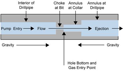
Figure PA- 21. Effective Wellbore Flow Geometry Before Bit Penetration

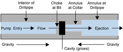
Figure PA- 22. Effective Wellbore Flow Geometry After Bit Penetration

Prior to drill bit penetration into the repository, gas from the repository can flow through drilling-damaged salt into the well. After penetration, the cavity at the bottom of the wellbore couples the wellbore flow and the repository flow models; gas and waste material can exit the repository domain into the cavity. The cavity radius increases as waste materials are moved into the wellbore.

The system of equations representing flow in the wellbore consists of four equations for mass conservation, one for each phase (salt, waste, mud, and gas); one equation for conservation of total momentum; two equations relating gas and mud density to pressure; the definition of density for the fluid mixture; and one constraint imposed by the fixed volume of the wellbore. The conservation of mass and momentum is described by

(PA.153)

(PA.154)

where

q = phase (w for waste, s for salt, m for mud, and g for gas)

V _q = volume (m³) of phase q

V = total volume (m³)

r _q = density (kg/m³) of phase q, constant for salt and waste (2,180 and 2,650 kg/m³, respectively) and pressure-dependent for gas and mud (see Equation (PA.155) and Equation (PA.156))

r = density of fluid mixture (kg/m³) determined by Equation (PA.157)

u = velocity (m/s) of fluid mixture in wellbore

t = time (s)

z = distance (m) from inlet at top of well

S _q = rate of mass (kg/s) in phase q entering and exiting wellbore domain at position z (Equation (PA.168))

S _mom = rate of momentum (kg m/s²) entering and exiting wellbore domain at position z (Equation (PA.171))

P = pressure (Pa) at position z

g = standard gravity (9.8067 kg/m/s²)

F = friction loss using pipe flow model (kg/m²/s²) determined by Equation (PA.159)

Gas is treated as isothermal and ideal, so the pressure and density are related by Boyle's law:

(PA.155)

where r _g _,0 is the density of H₂ gas at atmospheric pressure and 298 K (8.24182 ´ 10^-2 kg/m³).

The mud is assumed to be a compressible fluid, so

(PA.156)

where r _m _,0 is the density of the mud at atmospheric pressure (1,210 kg/m³) and c _m is the compressibility of the mud (3.1 ´ 10^-10 Pa^-1).

The density of the fluid mixture is determined from the densities and volumes occupied by the phases:

(PA.157)

The volume of each phase is constrained by the fixed total volume of the wellbore:

(PA.158)

The friction loss is a standard formulation for pipe flow (Fox and McDonald 1985), where the head loss per unit length is given as

(PA.159)

where the hydraulic diameter d _h is given by

(PA.160)

with D_i and D_o being the inner and outer diameters, respectively. In PA, D _o = 0.31115 m throughout the domain. From the bit to the top of the collar, D _i = 0.2032 m; above the collar, D _i = 0.1143 m. The area A is calculated as the area of the annulus between the outer and inner radii:

(PA.161)

Thus, d _h = 0.108 m from the bit to the top of the collar, and d _h = 0.197 m above the collar.

The Darcy friction factor f in Equation (PA.159) is determined by the method of Colebrook (Fox and MacDonald 1985). In the laminar regime, which is assumed to be characterized by Reynolds numbers below 2100 (Walker 1976),

(PA.162)

and in the turbulent regime (Re > 2100)

(PA.163)

where is the Reynolds number of the mixture, and h is the viscosity calculated in Equation (PA.164), below. As the wellbore mixture becomes particle-laden, the viscosity of the mixture is determined from an empirical relationship developed for proppant slurry flows in channels for the oil and gas industry (Barree and Conway 1995). Viscosity is computed by an approximate slurry formula based on the volume fraction of waste solids:

(PA.164)

where h ₀ is a base mixture viscosity (9.17 ´ 10^- ³ Pa s), w = V _w /V is the current volume fraction of waste solids, w _max is an empirically determined maximal volume fraction above which flow is choked (0.615), and s is an empirically determined constant (-1.5) (Hansen, Pfeifle, and Lord 2003).

PA-4.6.2.1.1 Wellbore Initial Conditions

Initial conditions in the wellbore approximate mixture flow conditions just prior to waste penetration. The wellbore is assumed to contain only mud and salt. Initial conditions for the pressure, fluid density, volume fractions of mud and salt, and the mixture velocity are set by the following algorithm:

Step 1. Set pressure in the wellbore to hydrostatic: P(z) = P _atm - r _m, ₀ gz.

Step 2. Set mud density using Equation (PA.156).

Step 3. Set mixture velocity: u(z) = R _m /A(z), where R _m is the volume flow rate of the pump (0.0202 m³/s), and A(z) is the cross-sectional area of the wellbore.

Step 4. Set volume of salt in each cell: V _s,i = R _drillA _bit D z _i /u _i , where R _drill is the rate of drilling (0.004445 m/s), is the area of the bottom of the wellbore, D z _i is the i-th zone size, u _i is the mixture velocity in the i-th zone, and d _bit is the diameter of the bit (0.31115 m).

Step 5. Set volume fraction of mud in each cell: V _m,i = V _i - V _s,i .

Step 6. Recalculate mixture density using Equation (PA.157), assuming no waste or gas in the wellbore.

The initial conditions set by this algorithm approximate a solution to the wellbore flow (Equation (PA.153) and Equation (PA.154)) for constant flow of mud and salt in the well. The approximation rapidly converges to a solution for wellbore flow if steady-state conditions are maintained (WIPP Performance Assessment 2003c).

PA-4.6.2.1.2 Wellbore Boundary Conditions

For simplicity, DRSPALL does not model flow of mud down the pipe to the bit. Mass can enter the wellbore below the drill bit and exit at the wellbore outlet. Below the bit, mud, salt, gas, and waste can enter the wellbore. PA assumes a constant volume of mud flow down the drilling pipe; therefore, the source term for mud, S _m,in , is set by the volumetric flow rate of the pump R _m (0.0202 m³/s) and the density of the mud at the bottom of the wellbore:

(PA.165)

Until the drill bit penetrates the repository, salt enters the wellbore at a constant rate:

(PA.166)

Additional mass enters the wellbore by gas flow from the repository (S _gas,in ) and spalling of waste material (S _w,in ); these mass sources are discussed in Section PA-4.6.2.3. The outlet of the wellbore is set to atmospheric pressure. Mass exiting the wellbore is determined from the mixture velocity, the area of the outlet A _out (0.066 m²), and the density and volume fraction of each phase at the outlet of the wellbore:

(PA.167)

Finally, the net change in mass and momentum for phase q is

(PA.168)

(PA.169)

The outlet of the wellbore is set to atmospheric pressure. Momentum exiting the wellbore is determined from the fluid velocity and the area of the outlet A _out (0.066 m²):

(PA.170)

No momentum is added by mass flow into the wellbore from the repository; thus

(PA.171)

PA-4.6.2.2 Repository Flow Model

The repository is modeled as a radially symmetric domain. A spherical coordinate system is used for most DRSPALL calculations. In a few circumstances, cylindrical coordinates are used in PA calculations, where spall volumes are large enough that spherical coordinates are not representative of the physical process (Lord, Rudeen, and Hansen 2003). The design document for DRSPALL (WIPP Performance Assessment 2003d) provides details on implementing the repository flow model in cylindrical coordinates.

Flow in the repository is transient, compressible, viscous, and single-phase (gas) flow in a porous medium. Gas is treated as isothermal and ideal. The equations governing flow in the repository are the equation of state for ideal gases (written in the form of Boyle's law for an ideal gas at constant temperature), conservation of mass, and Darcy's law with the Forchheimer correction (Aronson 1986, Whitaker 1996):

(PA.172)

(PA.173)

(PA.174)

where

P = pressure in pore space (Pa)

r _g = density of gas (kg/m³)

u = velocity of gas in pore space (m/s)

f = porosity of the solid (unitless)

h _g = gas viscosity (8.934 ´ 10^-6 Pa s)

k = permeability of waste solid (m²)

F = Forchheimer correction (unitless)

The Forchheimer correction is included in Equation (PA.174) to account for inertia in the flowing gas, which becomes important at high gas velocities (Ruth and Ma 1992). When the Forchheimer coefficient is zero, Equation (PA.174) reduces to Darcy's law. A derivation of Equation (PA.174) from the Navier-Stokes equations is given by Whitaker (1996); the derivation suggests that F is a linear function of gas velocity for a wide range of Reynolds numbers.

In PA, the Forchheimer correction takes the form

F = b _nd ru (PA.175)

where b _nd is the non-Darcy coefficient, which depends on material properties such as the tortuosity and area of internal flow channels, and is empirically determined (Belhaj et al. 2003). DRSPALL uses a value from Li et al. (2001) that measured high-velocity nitrogen flow through porous sandstone wafers, giving the result

(PA.176)

Equation (PA.172), Equation (PA.173) and Equation (PA.174) combine into a single equation for pressure in the porous solid:

(PA.177)

where

(PA.178)

and the Laplacian operator in a radially symmetric coordinate system is given by

(PA.179)

where n = 2 and n = 3 for polar and spherical coordinates, respectively.

In DRSPALL, the permeability of the waste solid is a subjectively uncertain parameter that is constant for waste material that has not failed and fluidized. In a region of waste that has failed, the permeability increases as the waste fluidizes by a factor of 1 + F _f , where F _f is the fraction of failed material that has fluidized and is based on the fluidization relaxation time. This approximately accounts for the material bulking as it fluidizes.

Initial pressure in the repository is set to a constant value P _ff . A no-flow boundary condition is imposed at the outer boundary (r = R):

Ñ P(R) = 0 (PA.180)

At the inner boundary (r = r _cav ), the pressure is specified as P(r _cav ,t) = P _cav (t), where P _cav (t) is defined in the next section. The cavity radius r _cav increases as drilling progresses and waste material fails and moves into the wellbore; calculation of r _cav is described in Section PA-4.6.2.3.3.

PA-4.6.2.3 Wellbore to Repository Coupling

Prior to penetration, a cylinder of altered-permeability salt material with diameter equal to the drill bit is assumed to connect the bottom of the wellbore to the repository. At the junction of the repository and this cylinder of salt, a small, artificial cavity is used to determine the boundary pressure for repository flow. After penetration, the cavity merges with the bottom of the wellbore to connect the wellbore to the repository.

PA-4.6.2.3.1 Flow Prior to Penetration

The cylinder of salt connecting the wellbore to the repository is referred to as the drilling damaged zone (DDZ) in Figure PA-19. The permeability of the DDZ, k _DDZ , is 1 ´ 10^-14 m². The spallings model starts with the bit 0.15 m above the repository; the bit advances at a rate of R _drill = 0.004445 m/s.

To couple the repository to the DDZ, the model uses an artificial pseudo-cavity in the small hemispherical region of the repository below the wellbore with the same surface area as the bottom of the wellbore (Figure PA-22). The pseudo-cavity is a numerical device that smoothes the discontinuities in pressure and flow that would otherwise occur upon bit penetration of the repository. The pseudo-cavity contains only gas, and is initially at repository pressure. The mass of gas in the cavity m _cav is given by

(PA.181)

where

S rep = gas flow from repository into pseudo-cavity (kg/s); see Equation (PA.182)

S g, in = gas flow from pseudo-cavity through DDZ into wellbore (kg/s); see Equation (PA.183)

Flow from the repository into the pseudo-cavity is given by

(PA.182)

where

r _g,rep = gas density in repository at cavity surface (kg/m³) =

u _rep = gas velocity (m/s) in repository at cavity surface =

f = porosity of waste (unitless)

A _cav = surface area of hemispherical part of the cavity (m²)

= , where d _bit is the diameter of the bit (m)

Flow out of the pseudo-cavity through the DDZ and into the wellbore is modeled as steady-state using Darcy's Law:

(PA.183)

where

h _g = viscosity of H₂ gas (8.934 ´ 10^- ⁶ Pa s)

M _w = molecular weight of H₂ gas (0.00202 kg / mol)

R = ideal gas constant (8.314 J/mol K)

T = repository temperature (constant at 300 K (27 ºC; 80 ºF))

L = length (m) of DDZ (from bottom of borehole to top of repository)

P _cav = pressure in pseudo-cavity (Pa)

P _BH = pressure at bottom of wellbore (Pa)

A justification for using this steady-state equation is provided in the design document for DRSPALL (WIPP Performance Assessment 2003d). The pseudo-cavity is initially filled with gas at a pressure of P _ff . The boundary pressure on the well side (P _BH ) is the pressure immediately below the bit, determined by Equation (PA.153) and Equation (PA.154). The pressure in the pseudo-cavity (P _cav ) is determined by the ideal gas law:

(PA.184)

where m _cav is the number of moles of gas in the cavity and the cavity volume V _cav is given by

(PA.185)

In PA, the drilling rate into the ground is assumed constant at 0.004445 m/s; thus L = L _i - 0.004445t until L = 0, at which time the bit penetrates the waste. The term L _i is the distance from the bit to the waste at the start of calculation (0.15 m).

PA-4.6.2.3.2 Flow After Penetration

After waste penetration, the bottom of the wellbore is modeled as a hemispherical cavity in the repository, the radius of which grows as drilling progresses and as material fails and moves into the cavity. Gas, drilling mud, and waste are assumed to thoroughly mix in this cavity; the resulting mixture flows around the drill collars and then up the annulus between the wellbore and the drill string. Gas flow from the repository into the cavity is given by Equation (PA.182); however, A _cav is now dependent on the increasing radius of the cavity (see Section PA-4.6.2.3.3). Mudflow into the cavity from the wellbore is given by Equation (PA.165). Waste flow into the cavity is possible if the waste fails and fluidizes; these mechanisms are discussed in Section PA-4.6.2.3.4 and Section PA-4.6.2.3.5. Pressure in the cavity is equal to that at the bottom of the wellbore, and is computed by Equation (PA.184).

PA-4.6.2.3.3 Cavity Volume After Penetration

The cylindrical cavity of increasing depth created by drilling is mapped to a hemispherical volume at the bottom of the wellbore to form the cavity. This mapping maintains equal surface areas in order to preserve the gas flux from the repository to the wellbore. The cavity radius from drilling is thus

(PA.186)

where D H is the depth of the drilled cylinder. In PA, the drilling rate into the ground is assumed constant at 0.004445 m/s; thus D H = 0.004445t until D H = H, the height of compacted waste (m). Since the initial height of the repository is 3.96 m, H is computed from the porosity f by , where f ₀ is the initial porosity of a waste-filled room.

The cavity radius r _cav is increased by the radius of failed and fluidized material r _fluid , which is the depth to which fluidization has occurred beyond the drilled radius. That is,

(PA.187)

PA-4.6.2.3.4 Waste Failure

Gas flow from the waste creates a pressure gradient within the waste, which induces elastic stresses in addition to the far-field confining stress. These stresses may lead to tensile failure of the waste material, an assumed prerequisite to spallings releases. While the fluid calculations using Equation (PA.172), Equation (PA.173) and Equation (PA.174) are fully transient, the elastic stress calculations are assumed to be quasi-static (i.e., sound-speed phenomena in the solid are ignored). Elastic effective stresses are (Jaeger and Cook 1969)

(PA.188)

(PA.189)

where b is Biot's constant (assumed here to be 1.0) and s _ff is the confining far-field stress (assumed constant at 14.8 MPa).

The flow-related radial and tangential stresses ( s _sr and s _s _q , respectively) are computed by equations analogous to differential thermal expansion (Timoshenko and Goodier 1970):

(PA.190)

(PA.191)

where P _ff is the initial repository pressure and u is Poisson's ratio (0.38).

Since stresses are calculated as quasi-static, an initial stress reduction caused by an instantaneous pressure drop at the cavity face propagates instantaneously through the waste. The result of calculating Equation (PA.188) can be an instantaneous early-time tensile failure of the entire repository if the boundary pressure is allowed to change suddenly. This is nonphysical and merely a result of the quasi-static stress assumption, combined with the true transient pore pressure and flow-related stress equations. To prevent this nonphysical behavior, tensile failure propagation is limited by a tensile failure velocity (1000 m/s; see Hansen et al. 1997). This limit has no quantitative effect on results, other than to prevent nonphysical tensile failure.

At the cavity face, Equation (PA.188) and Equation (PA.190) evaluate to zero, consistent with the quasi-static stress assumption. This implies that the waste immediately at the cavity face cannot experience tensile failure; however, tensile failure may occur at some distance into the waste material. Consequently, the radial effective stress s _r is averaged from the cavity boundary into the waste over a characteristic length L _t (0.02 m). If this average radial stress is tensile and its magnitude exceeds the material tensile strength (| | > TENSLSTR), the waste is no longer capable of supporting radial stress and fails, permitting fluidization. The waste tensile strength is an uncertain parameter in the analysis (see TENSLSTR in Table PA-11).

Equation (PA.189) and Equation (PA.191) evaluate shear stresses in the waste. DRSPALL does not use the waste shear stresses to calculate waste failure for spall releases. These stresses are included in this discussion for completeness.

PA-4.6.2.3.5 Waste Fluidization

Failed waste material is assumed to be disaggregated, but not in motion; it remains as a porous, bedded material lining the cavity face, and is treated as a continuous part of the repository from the perspective of the porous flow calculations. The bedded material may be mobilized and enter the wellbore if the gas velocity in the failed material (see Equation (PA.174)) exceeds a minimum fluidization velocity, U _f . The minimum fluidization velocity is determined by solving the following quadratic equation (Cherimisinoff and Cherimisinoff 1984, Ergun 1952)

(PA.192)

where

a = particle shape factor (unitless)

d p = particle diameter (m)

Fluidization occurs in the failed material to the depth at which gas velocity does not exceed the fluidization velocity; this depth is denoted by r _fluid and is used to determine cavity radius (Section PA-4.6.2.3.3). If fluidization occurs, the gas and waste particles mix into the cavity at the bottom of the wellbore. Because this mixing cannot be instantaneous, which would be nonphysical (much as allowing instantaneous tensile failure propagation would be nonphysical), a small artificial relaxation time, equal to the cavity radius r _cav divided by the superficial gas velocity u(r _cav ), is imposed upon the mixing phenomenon. The fluidized material is released into the cavity uniformly over the relaxation time.

PA-4.6.3 Numerical Model

The numerical model implements the conceptual and mathematical models described above (Section PA-4.6.2). Both the wellbore and the repository domain calculations use time-marching finite differences. These are part of a single computational loop and therefore use the same time step. The differencing schemes for the wellbore and repository calculations are similar, but not identical.

PA-4.6.3.1 Numerical Method-Wellbore

The wellbore is zoned for finite differencing, as illustrated in Figure PA-23, which shows zones, zone indices, grid boundaries, volumes, and interface areas. The method is Eulerian: zone boundaries are fixed, and fluid flows across the interfaces by advection. Quantities are zone-centered and in tegration is explicit in time.

To reduce computation time, an iterative scheme is employed to update the wellbore flow solution. The finite-difference scheme first solves Equation (PA.153) and Equation (PA.154) for the mass of each phase in each grid cell and the momentum in each grid cell.

The updated solution to Equation (PA.153) and Equation (PA.154) is then used to compute the volume of each phase, the pressure, and the mixture velocity in each grid cell.

All of the materials (mud, salt, gas, and waste) are assumed to move together as a mixture. Because fluid moves through the cell boundaries, the calculation requires a value for the flow through each cell boundary during a time step. These values are obtained by averaging the fluid velocities at the zone centers, given by

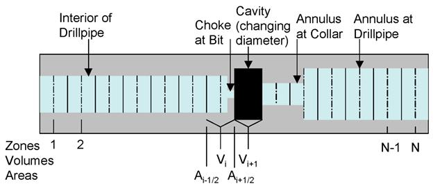
Figure PA- 23. Finite-Difference Zoning for Wellbore

(PA.193)

The mass transport equation, prior to any volume change, becomes

(PA.194)

Here, the source terms S _m,i correspond to material entering or exiting at the pump, cavity, and surface. The "upwind" zone-centered densities are used for the interfaces values, and .

Finally, any changed volumes are incorporated and numerical mass diffusion is added for stability:

(PA.195)

where

and z _q is the diffusion coefficient for phase q. The density r f _q for phase q being diffused is calculated from the mixture density, r , and the mass fraction, f _q , of phase q in the referenced cell (f _q = r V _q,i / r V _i ). The numerical diffusion coefficient z _q is chosen empirically for stability. Separate diffusion coefficients could be used for the different materials (mud, gas, etc.); however, sufficient stability is obtained by diffusing only mud and salt using the same coefficient ( z _m = z _s = 0.0001 and z _w = z _g = 0).

Momentum is differenced as

(PA.196)

where the dissipation term is obtained from Equation (PA.159) and is constrained by

(PA.197)

and the sign of is chosen to oppose flow. Finally, numerical momentum diffusion is added without distinguishing between phases in the mixture ( r is the mixture density):

(PA.198)

In PA, z _p = 0.01.

Equation (PA.156), Equation (PA.157), and Equation (PA.158) comprise a simultaneous system of equations for the volumes of gas and mud and the pressure in the wellbore. The volumes of salt and waste are known, since they are considered incompressible. Equation (PA.156) and Equation (PA.157) combine into a quadratic equation for gas volume:

(PA.199)

where

The volume of the mud phase follows from Equation (PA.156) and the pressure from Equation (PA.155). Once the mixture density in each cell ( r _i ) is updated by Equation (PA.157), the mixture velocity in each cell (u _i ) is computed by

(PA.200)

where the quantity ru is determined by Equation (PA.198).

PA-4.6.3.2 Numerical Method-Repository

The time integration method for the repository flow is implicit, with spatial derivatives determined after the time increment. This method requires the inversion of a matrix for the entire repository, which is usually straightforward. The implicit scheme is unconditionally stable. However, it is still necessary to use small time steps to ensure gradient accuracy.

The numerical method follows Press et al. (1989). For simplicity, the equations are presented for constant zone size, although DRSPALL implements difference equations that allow for a variable zone size. Near the cavity, a small, constant zone size is used, and then zones are allowed to grow geometrically as the outer boundary is approached. This procedure greatly increases computational efficiency without sacrificing accuracy in the region of interest.

For an isothermal ideal gas, the pseudopressure y is defined as

(PA.201)

Using Equation (PA.201), Equation (PA.177) is expanded to

(PA.202)

where ; Equation (PA.202) is then converted to a difference equation by treating D( y ) as constant over a zone, using its zone-centered value at the current time :

(PA.203)

Collecting similar terms in y leads to a tridiagonal system:

, j = 1,2…. (PA.204)

where

Equation (PA.204) may be solved by simplified LU decomposition, as presented in Press et al. (1989).

The boundary condition at the inner radius is implemented by noting that for i = 1 (the first intact or nonfluidized cell), is the cavity pseudopressure, which is known, and therefore can be moved to the right-hand side of Equation (PA.204):

(PA.205)

The far-field boundary condition is a zero gradient, which is implemented by setting in Equation (PA.205), recognizing that and rearranging, which gives

(PA.206)

where j is the index of the last computational cell.

PA-4.6.3.3 Numerical Method-Wellbore to Repository Coupling

The term u _rep , appearing in Equation (PA.182), is the gas velocity in the repository at the waste-cavity interface and is determined from the pressure gradient inside the waste. DRSPALL uses the pressure (P1) at the center of the first numerical zone in the waste to determine u _rep :

(PA.207)

PA-4.6.4 Implementation in the PA

During development of the spallings model, a total of five parameters were determined to be both uncertain and potentially significant to model results (Hansen, Pfeifle, and Lord 2003; Lord and Rudeen 2003). All five parameters relate to the repository conditions or the state of the waste at the time of intrusion. Table PA-11 lists the uncertain parameters in the DRSPALL calculations; these parameters are also listed in Table PA-17.

Table PA- 11. Uncertain Parameters in the DRSPALL Calculations

Quantity	Property	Implementation
Repository Pressure	REPIPRES	Initial repository pressure (Pa); spall calculated for values of 10, 12, 14, and 14.8 MPa. Defines initial repository pressure in Equation (PA.177) (see Section PA-4.6.2.2) and P _ff in Equation (PA.190).
Repository Permeability	REPIPERM	Permeability (m²) of waste, implemented by parameter SPALLMOD/REPIPERM. Log-uniform distribution from 2.4 ´ 10^-14 to 2.4 ´ 10^-12. Defines k in Equation (PA.174).
Repository Porosity	REPIPOR	Porosity (dimensionless) of waste, implemented by parameter SPALLMOD/REPIPOR. Uniform distribution from 0.35 to 0.66. Defines f in Equation (PA.173).
Particle Diameter	PARTDIAM	Particle diameter of waste (m) after tensile failure, implemented by parameter SPALLMOD/PARTDIAM. Log-uniform distribution from 0.001 to 0.1 (m). Defines d _p in Equation (PA.192 ).
Tensile Strength	TENSLSTR	Tensile strength of waste (Pa), implemented by parameter SPALLMOD/TENSLSTR. Uniform distribution from 0.12 MPa to 0.17 MPa. Defines maximum for Section PA-4.6.2.3.4.

The computational requirements of DRSPALL prohibit calculation of spall volumes for all possible combinations of initial conditions and parameter values. Since repository pressure is a time-dependent value computed by the BRAGFLO model (see Section PA-4.2), DRSPALL calculations were performed for a small number of pressures. Sensitivity studies showed that spall does not occur at pressures below 10 MPa; this value was used as the lower bound on pressure. In DRSPALL, the repository pressure cannot exceed the far-field confining stress (14.8 MPa); consequently, 14.8 MPa was used as the upper bound on pressure. Computations were also performed for intermediate pressures of 12 and 14 MPa. The remaining four parameters listed in Table PA-11 are treated as subjectively uncertain. The uncertainty represented by these parameters pertains to the future state of the waste, which is modeled in PA as a homogeneous material with uncertain properties (see Section PA-5.0).

Spall volumes are computed for each combination of initial pressure and sample element, for a total of 4 ´ 300 = 1,200 model runs. Although repository porosity could be treated as an initial condition (using the time-dependent value computed by BRAGFLO), to reduce the number of computational cases and ensure that extreme porosity values were represented, repository porosity was included as a sampled parameter.

The spallings submodel of the code CUTTINGS_S uses the DRSPALL results to compute the spall volume for a given initial pressure P. If P < 10 MPa or P > 14.8 MPa, the spall volume is the value computed for REPIPRES = 10 MPa or REPIPRES = 14.8 MPa, respectively. If P falls between 10 and 14.8 MPa, the spall volume is constructed by linear interpolation between the DRSPALL results for pressures that bracket P.

PA-4.6.5 Additional Information

Additional information on DRSPALL and its use in PA to determine spallings releases can be found in the DRSPALL user's manual (WIPP Performance Assessment 2003e) and in the analysis package for spallings releases (Kicker 2013). Additional information on the construction of spall volumes by the code CUTTINGS_S can be found in the CUTTINGS_S design document (WIPP Performance Assessment 2003f).

PA-4.7 DBR to Surface: BRAGFLO

This section describes the model for DBR volumes, which are volumes of brine released to the surface at the time of a drilling intrusion. DBR volumes are calculated by the code BRAGFLO, the same code used to compute two-phase flow in and around the repository (see Section PA-4.2).

PA-4.7.1 Overview of Conceptual Model

DBRs could occur if the pressure in the repository at the time of a drilling intrusion exceeds 8 MPa, which is the pressure exerted by a column of brine-saturated drilling fluid at the depth of the repository (Stoelzel and O'Brien 1996). For repository pressures less than 8 MPa, no DBRs are assumed to occur. However, even if the repository pressure exceeds 8 MPa at the time of a drilling intrusion, a DBR is not assured, as there might not be sufficient mobile brine in the repository to result in movement towards the borehole. Brine saturation in the repository must exceed the residual brine saturation of the waste material. The residual brine saturation is sampled from a uniform distribution ranging from 0.0 to 0.552 in the CRA-2014 PA.

DBRs are estimated for the following cases: (1) an initial intrusion into the repository into either a lower (down-dip), middle, or upper (up-dip) panel; (2) an intrusion into a waste panel preceded by an E1 intrusion into either the same waste panel, an adjacent panel, or a nonadjacent panel; and (3) an intrusion into a waste panel preceded by an E2 intrusion into either the same waste panel, an adjacent panel, or a nonadjacent panel (see Section PA-6.7). To determine releases for the above cases, the DBR calculations use a computational grid that explicitly includes all 10 waste panels (Figure PA-24).

For perspective, the following list provides a comparison of the BRAGFLO mesh for the Salado flow calculations (Figure PA-12) and the DBR mesh used for the DBR calculations (Figure PA-24):

1. The DBR mesh is defined in the areal plane with the z dimension (height) one element thick; the BRAGFLO mesh is defined as a cross section, with multiple layers in height and the thickness (y dimension) one element thick.

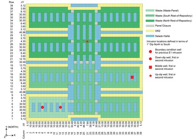
Figure PA- 24. DBR Grid Used in PA

2. The DBR mesh uses constant thickness, while the BRAGFLO mesh uses rectangular flaring to account for three-dimensional volumes in a two-dimensional grid (Figure PA-13).

3. The DBR mesh represents flow only in the waste area. The BRAGFLO model includes the surrounding geology as well as the entire WIPP excavation (including operations, experimental, and shaft regions).

4. Local scale heterogeneities are included in the DBR mesh, including the salt pillars, rooms, panel closures, and passageways that contain waste. These are not fully represented in the BRAGFLO mesh.

5. The DRZ is included in both models, but exists above and below the excavated regions in the BRAGFLO model, whereas the DRZ surrounds the waste rooms on the sides of the DBR mesh.

6. Both models include a one-degree formation dip through the excavated regions (Equation (PA.33)).

The DBRs are assumed to take place over a relatively short period of time (i.e., 3 to 4.5 days; see Section PA-4.7.8) following the drilling intrusion. The initial value conditions for determining DBR volumes are obtained by mapping solutions of Equation (PA.24), Equation (PA.25), Equation (PA.26), Equation (PA.27), Equation (PA.28), Equation (PA.29), and Equation (PA.30) obtained from BRAGFLO with the computational grid in Figure PA-12 onto the grid in Figure PA-24.

In concept, theDBR for a drilling intrusion has the form

(PA.208)

where

DBR = DBR volume (m³) for drilling intrusion

= rate (m³) at time t at which brine flows up intruding borehole

t = elapsed time (s) since drilling intrusion

t e = time (s) at which DBR ends

The definition of rDBR(t) is discussed in the following sections. It is based on the two-phase flow relationships in Equation (PA.24), Equation (PA.25), Equation (PA.26), Equation (PA.27), Equation (PA.28), Equation (PA.29), and Equation (PA.30) and use of the Poettmann-Carpenter correlation (Poettmann and Carpenter 1952) to determine a boundary pressure at the connection between the intruding borehole and the repository. The time t _e is based on current drilling practices in the Delaware Basin (Section PA-4.7.8).

PA-4.7.2 Linkage to Two-Phase Flow Calculation

The mesh in Figure PA-24 was linked to the mesh in Figure PA-12 by subdividing the waste disposal area in the mesh in Figure PA-12 into three regions (Figure PA-25). The upper region represents the northern rest of repository (North RoR) area in Figure PA-12. The middle region represents the southern rest of repository (South RoR) area in Figure PA-12. The lower region represents the farthest down-dip repository area (Waste Panel) in Figure PA-12 that contained waste and thus corresponds to the single down-dip waste panel. The linkage between the solutions to Equation (PA.24), Equation (PA.25), Equation (PA.26), Equation (PA.27), Equation (PA.28), Equation (PA.29), and Equation (PA.30) and the DBR calculations was made by assigning quantities calculated by BRAGFLO for each region in Figure PA-12 to the corresponding waste region in Figure PA-24.

The height of the grid in Figure PA-24 was assigned a value that corresponded to the crushed height, h (m), of the waste as predicted by the solution of Equation (PA.24), Equation (PA.25), Equation (PA.26), Equation (PA.27), Equation (PA.28), Equation (PA.29) and Equation (PA.30). Specifically,

(PA.209)

where h _i and f _i are the initial height (m) and porosity of the waste and f is the volume-averaged porosity of the waste at the particular time under consideration (Section PA-4.2.3). The areas designated panel closures, DRZ, and impure halite in Figure PA-24 were assigned the same pressures and saturations as the corresponding grid blocks in the 10,000-year BRAGFLO calculations. Moreover, panel closure areas in the DBR calculation were assigned the same porosity and permeability values as the corresponding grid blocks in the 10,000-year BRAGFLO calculation.

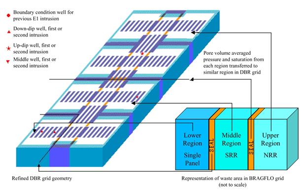
Figure PA- 25. Assignment of Initial Conditions for DBR Calculation

The initial brine pressure p _b (x, y, 0) and gas saturation S _g (x, y, 0) in the grid in Figure PA-24 are assigned by

(PA.210)

(PA.211)

where designates a point in the grid in Figure PA-24, and denote solutions to Equation (PA.24), Equation (PA.25), Equation (PA.26), Equation (PA.27), Equation (PA.28), Equation (PA.29), and Equation (PA.30), and denote the variables of integration, t _int is the time at which the drilling intrusion occurs, and R corresponds to the region in the BRAGFLO computational grid (Figure PA-12) that is mapped into the region in the DBR computational grid (Figure PA-24) that contains the point (x, y) (Figure PA-25). Note that t _int defines a time in the solution of Equation (PA.24), Equation (PA.25), Equation (PA.26), Equation (PA.27), Equation (PA.28), Equation (PA.29), and Equation (PA.30); t = 0 defines the start time for the DBR calculation and corresponds to t _int in the solution of Equation (PA.24), Equation (PA.25), Equation (PA.26), Equation (PA.27), Equation (PA.28), Equation (PA.29), and Equation (PA.30).

The initial porosity f (x, y, 0) of DRZ regions in the DBR grid (Figure PA-24) is set by the equation listed in Table PA-12. In Table PA-12, h(t _int ) is the height of the repository at the time of intrusion (typically 1 to 1.5 m; corresponds to h in Equation (PA.24), Equation (PA.25), Equation (PA.26), Equation (PA.27), Equation (PA.28), Equation (PA.29), and Equation (PA.30)), h _DRZ,i is the effective DRZ height (43.50 m) that results in the DRZ in Figure PA-24 having the same pore volume as the initial pore volume of the DRZ in Figure PA-12, and f _DRZ,i is the initial porosity of the DRZ (see Table PA-3). The initial porosities of panel closure and Salado halite regions are set to their corresponding values in the 10,000-year BRAGFLO run at the time of intrusion. The initial porosity of waste regions in the DBR grid is set to the average porosity of the intruded panel, the south rest-of-repository, and the north rest-of-repository at the time of intrusion.

Table PA- 12. Initial DRZ Porosity in the DBR Calculation

Grid Region	Initial Porosity
DRZ

PA-4.7.3 Conceptual Representation for Flow Rate rDBR(t)

The driving force that would give rise to the DBR is a difference between waste panel pressure, p _w (Pa), and the flowing bottomhole pressure in the borehole, p _wf (Pa), at the time of the intrusion. The flowing bottomhole pressure p _wf , defined as the dynamic pressure at the inlet of the intruding borehole to the waste panel, is less than the static pressure p _w due to friction and acceleration effects. The rate at which brine and gas are transported up the intruding borehole is determined by the difference p _w - p _wf and a productivity index J _p for the intruded waste panel (Mattax and Dalton 1990, p. 79):

(PA.212)

where

= flow rate (m³/s) at time t for phase p (p = b ~ brine, p = g ~ gas)

= productivity index (m³/Pa·s) for phase p

and p _w and p _wf are defined above. As indicated by the inclusion/exclusion of a dependence on t, the terms J _p and p _wf are constant during the determination of q _p (t) for a particular drilling intrusion in the present analysis, and p _w (t) changes as a function of time. In concept, the DBR is given by

(PA.213)

once J _b (brine), p _w , and p _wf are determined. Section PA-4.7.4 discusses the determination of J _p (for both gas and brine), Section PA-4.7.5 presents the numerical determination of p _w and DBR, and the determination of p _wf is discussed in Section PA-4.7.6. The associated gas release is given by the corresponding integral with J _g (gas) rather than J _b (brine). In the computational implementation of the analysis, DBR is determined as part of the numerical solution of the system of PDEs that defines p _w (Section PA-4.7.5).

PA-4.7.4 Determination of Productivity Index Jp

In a radial drainage area with uniform saturation, which is assumed to be valid throughout the DBR, the following representation for J _p can be determined from Darcy's law (Mattax and Dalton 1990, p. 79; Williamson and Chappelear 1981; Chappelear and Williamson 1981):

(PA.214)

where

k = absolute permeability (assumed to be constant through time at 2.4 ´ 10^- ¹³ m²)

k rp = relative permeability to phase p (calculated with modified Brooks-Corey model in Equation (PA.145), Equation (PA.146), and Equation (PA.147) and brine and gas saturations, S b and S g , obtained by mapping solutions of Equation (PA.24), Equation (PA.25), Equation (PA.26), Equation (PA.27), Equation (PA.28), Equation (PA.29), and Equation (PA.30) obtained with the grid in Figure PA-12 onto the grid in Figure PA-24)

h = crushed panel height (Equation (PA.209))

m p = viscosity of fluid phase (assumed to be constant through time with m b = 1.8 ´ 10^- ³ Pa·s, and m g = 8.92 ´ 10^- ⁶ Pa·s [Kaufmann 1960])

r e = external drainage radius (for use with the rectangular grid blocks in Figure PA-24, r e is taken to be the equivalent areal radius; see Equation (PA.215))

r w = wellbore radius (assumed to be constant through time at 0.1556 m (Gatlin 1960, Table 14.7)

c = -0.50 for pseudo-steady-state flow

s = skin factor, which is used to incorporate flow stimulation caused by cavings and spallings release (see Equation (PA.216))

In the present analysis,

(PA.215)

where D x is the x dimension (m) and D y is the y dimension (m) of the grid block containing the down-dip well in Figure PA-24 (D x = 10 m and D y = 30.5 m).

The skin factor s is derived from the cavings and spallings release. Due to the uncertainty in the cavings and spallings parameters, the calculated solid release volume can vary for each realization. The skin factor is calculated for each realization, based on the calculated solid release volume, through the following petroleum engineering well testing relationship (Lee 1982, pp. 5-7):

(PA.216)

where

k s = permeability (m²) of an open channel as a result of spallings releases (assumed to be infinite)

r s = effective radius (m) of the wellbore with the cuttings, cavings, and spallings volume removed

The effective radius r _s is obtained by converting the cuttings, cavings, and spallings volume removed into a cylinder of equal volume with the initial height of the waste (h _i ), and then computing the radius of the cylinder:

(PA.217)

and substitution of r _s into Equation (PA.216) with k _s = ¥ yields

(PA.218)

PA-4.7.5 Determination of Waste Panel Pressure pw(t) and DBR

The repository pressure p _w (t) in Equation (PA.213) after a drilling intrusion is determined with the same system of nonlinear PDEs discussed in Section PA-4.2. These equations are solved numerically by the code BRAGFLO used with the computational grid in Figure PA-24 and assumptions (i.e., parameter values, initial value conditions, and boundary value conditions) appropriate for representing brine flow to an intruding borehole over a relatively short time period immediately after the intrusion (e.g., 3 to 4.5 days). Due to the short time periods under consideration, the model for DBR does not include gas generation due to either corrosion or microbial action or changes in repository height due to creep closure.

Although the determination of DBR can be conceptually represented by the integral in Equation (PA.208), in the numerical implementation of the analysis, DBR is determined within the numerical solution of the system of PDEs that defines p _b (x, y, t).

With the specific assumptions for DBR, Equation (PA.24) , Equation (PA.25), Equation (PA.26), Equation (PA.27), Equation (PA.28), Equation (PA.29), and Equation (PA.30) become

Gas Conservation Ñ × (PA.219)

Brine Conservation Ñ × (PA.220)

Saturation Constraint (PA.221)

Capillary Pressure Constraint (PA.222)

Gas Density r _g determined by RKS equation of state (Equation (PA.52)) (PA.223)

Brine Density (PA.224)

Formation Porosity (PA.225)

with all symbols having the same definitions as in Equation (PA.24), Equation (PA.25), Equation (PA.26) Equation (PA.27), Equation (PA.28), Equation (PA.29), and Equation (PA.30).

The primary differences between the BRAGFLO calculations described in Section PA-4.2 and the BRAGFLO calculations described in this section are in the computational meshes (Figure PA-24 and Figure PA-12), initial values (Table PA-3 and Section PA-4.7.2), and boundary conditions (Table PA-13). In particular, brine and gas flow associated with intruding boreholes in the DBR calculations are incorporated by the assignment of appropriate boundary conditions. Specifically, brine flow up an intruding borehole is incorporated into Equation (PA.219), Equation (PA.220), Equation (PA.221), Equation (PA.222), Equation (PA.223), Equation (PA.224), and Equation (PA.225) by using the Poettmann-Carpenter wellbore model to determine the pressure at the outflow point in a waste panel (Figure PA-24), with this pressure entering the calculation as a boundary value condition (Table PA-13). The details of this determination are discussed in Section PA-4.7.6. Furthermore, for calculations that assume a prior E1 intrusion, the effects of this intrusion are also incorporated into the analysis by specifying a pressure as a boundary condition (Table PA-13). The determination of this pressure is discussed in Section PA-4.7.6.

Table PA- 13. Boundary Conditions for p _b and S _g in DBR Calculations

on Upper (Northern) or Lower (Southern) Boundary in Figure PA-24, t ≥ 0
× j = 0 Pa/m	No gas flow condition
× j = 0 Pa/m	No brine flow condition
on Right (Eastern) or Left (Western) Boundary in Figure PA-24, t ≥ 0
× i = 0 Pa/m	No gas flow condition
× i = 0 Pa/m	No brine flow condition
at Location of Drilling Intrusion under Consideration (see indicated points in Figure PA-24), t ≥ 0
(see Section PA-4.7)	Constant pressure condition
at Location of Prior Drilling Intrusion into Pressurized Brine (see indicated point in Figure PA-24), t ≥ 0
(see Section PA-4.7.7)	Constant pressure condition

PA-4.7.6 Boundary Value Pressure pwf

The boundary value pressure p _wf at the inlet of the intruding borehole is defined by a system of equations of the following form:

(PA.226)

(PA.227)

(PA.228)

(PA.229)

where p(h) is pressure (Pa) at elevation h in the borehole, with h = 0 m corresponding to the entry point of the borehole into the waste panel and h = 655 m corresponding to the land surface (Figure PA-26); G is a function (Pa/m) characterizing the change of pressure with elevation in the borehole; p(655) is an initial value condition requiring that pressure at the land surface (i.e., the outlet point of the borehole) be equal to atmospheric pressure; q _b [p(0)] and q _g [p(0)] define brine and gas flow rates (m³/s) into the borehole; J _b and J _g are productivity indexes (m³/Pa s) (see Equation (PA.214); and p _w is the pressure (Pa) in the repository at the time of the drilling intrusion.

Figure PA- 26. Borehole Representation Used for Poettmann-Carpenter Correlation

The boundary value pressure p _wf is defined by

(PA.230)

Thus, p _wf is determined by the numerical solution of Equation (PA.226) for p(0) subject to the constraints in Equation (PA.227), Equation (PA.228), and Equation (PA.229).

The pressure p _w corresponds to the pressure p _w (0), and is obtained from the solution of Equation (PA.24), Equation (PA.25), Equation (PA.26), Equation (PA.27), Equation (PA.28), Equation (PA.29), and Equation (PA.30) with the computational grid in Figure PA-12 (see Section PA-4.7.2). The production indexes J _b and J _g are defined in Equation (PA.214). Thus, the only quantity remaining to be specified in Equation (PA.226), Equation (PA.227), Equation (PA.228), and Equation (PA.229) is the function G.

Brine and gas flow up a borehole is governed by complex physics dependent on frictional effects and two-phase fluid properties. This phenomenon has been widely studied in the petroleum industry and many modeling procedures have been developed to predict flow rates and pressures in vertical two-phase pipe flow (i.e., to define G in Equation (PA.226)) (Brill and Beggs 1986). For this analysis, the Poettmann-Carpenter model (Poettmann and Carpenter 1952; Welchon, Bertuzzi, and Poettmann 1962) was used to define G because it accounts for multiphase frictional effects based on empirical (i.e., field) data from flowing wells, is one of the few modeling approaches that included annular flow data in its development, and is relatively easy to implement. Specifically, the Poettmann-Carpenter model defines G by

(PA.231)

where

g = acceleration due to gravity (9.8 m/s²)

m(h) = density (kg/m³) of fluids (i.e., gas and brine) in wellbore at elevation h (Note: m(h) is a function of q _b[p(0)] and q _g[p(0)]; see Equation (PA.232))

= empirically defined scale factor (m/s²) (Note: f ¢ is the scale factor in the Poettmann-Carpenter model for fluid flow in a wellbore [Poettmann and Carpenter 1952]; see discussion below)

= flow rate (m³/s) of fluids (i.e., gas and brine) in wellbore at elevation h (Note: F(h) is a function of q _b[p(0)] and q _g[p(0)]; see Equation (PA.233))

= effective diameter (m) of wellbore (see Equation (PA.236))

The first term, gm(h), in Equation (PA.231) results from the contribution of elevation to pressure; the second term results from frictional effects (Poettmann and Carpenter 1952). The fluid density m(h) at elevation h is given by

(PA.232)

where

(PA.233)

and

= density (kg/m³) of brine at pressure p(0) and temperature 300.1 K, which is fixed at 1230 kg/m³

= density (kg/m³) of H₂ at pressure p(0) and temperature 300.1 K (see Equation (PA.234))

= z-factor for compressibility of H₂ at elevation h (Note: z(h) is a function of p(h); see Equation (PA.235)), and q _b[p(0)] and q _g[p(0)] are defined in Equation (PA.226), Equation (PA.227), Equation (PA.228), and Equation (PA.229)

The gas density in Equation (PA.232) is obtained from the universal gas law, , by

(PA.234)

where n is the amount of gas (mol) in a volume V, C _m,kg is the conversion factor from moles to kilograms for H₂ (i.e., 2.02 ´ 10^- ³ kg/mol), P = p(0), R = 8.3145 J/mol K, and T = 300.1 K. The z-factor is given by

(PA.235)

and was obtained from calculations performed with the SUPERTRAPP program (Ely and Huber 1992) for pure H₂ and a temperature of 300.1 K (Stoelzel and O'Brien 1996, Figure 4.7.4). The preceding approximation to z(h) was obtained by fitting a straight line between the results for pressures of 0 psi and 3000 psi and a H₂ mole fraction of 1 in Stoelzel and O'Brien (1996, Figure 4.7.4); the actual calculations used the more complex, but numerically similar, regression model given in Stoelzel and O'Brien (1996, Figure 4.7.4). The numerator and denominator in Equation (PA.232) involve rates, with the time units canceling to give m(h) in units of kg/m³.

The effective diameter D(h) in Equation (PA.231) is defined with the hydraulic radius concept. Specifically,

(PA.236)

where D _i (h) and D _o (h) are the inner and outer diameters (m) of the wellbore at elevation h(m) (see Figure PA-26). The factor in Equation (PA.231) is a function of m(h), D(h), and q _b [p(0)].

Subsequent to submittal of the CCA PA, it was discovered that the factor of was omitted from Equation (PA.214). This error was determined to be of no consequence to the CCA PA conclusions (Hadgu et al. 1999) and was corrected in the CRA-2004 PA. As a consequence of the error correction, the regression models used to determine the boundary pressure p _wf were recalculated (Hadgu et al. 1999). The corrected regression models are reported in this appendix.

The following iterative procedure based on the bisection method was used to approximate solutions to Equation (PA.226), Equation (PA.227), Equation (PA.228), and Equation (PA.229).

Step 1. Estimate p(0) using a bisection algorithm:

The initial guess for p(0) is the midpoint of interval [0, p _w], where p _w is the pressure in the repository at the time of the drilling intrusion used in Equation (PA.226), Equation (PA.227), Equation (PA.228), and Equation (PA.229).

The next guess for p(0) is at the midpoint of either or , depending on whether the resultant approximation to p(655) is above or below atmospheric pressure.

Subsequent guesses for p(0) are made in a similar manner.

Step 2. Use p(0), known values for J _b, J _g, and p _w, and Equation (PA.226), Equation (PA.227), Equation (PA.228), and Equation (PA.229) to determine q _b[p(0)] and q _g[p(0)].

Step 3. Use the bisection method with D h = 25 ft = 7.62 m and appropriate changes in annular diameter (Figure PA-26) to determine p(655) (i.e., p(h + D h) = p(h) + G(q _b[p(0)], q _g[p(0)], p(h), h), D h)).

Step 4. Stop if p(655) is within 0.07% of atmospheric pressure (i.e., if |1.013×10⁵ Pa -p(655)| £ 70 Pa)). Otherwise, return to Step 1 and repeat process.

The preceding procedure is continued until the specified error tolerance (i.e., 0.07%) has been met. The computational design of the PA has the potential to require more than 23,000 separate DBR calculations (3 replicates ´ 5 scenarios ´ 3 drilling locations ´ 100 vectors ´ 5 to 6 intrusion times per scenario). In concept, each of these cases requires the solution of Equation (PA.226), Equation (PA.227), Equation (PA.228), and Equation (PA.229) with the iterative procedure just presented to obtain the boundary value condition p _wf = p(0) (Table PA-13). To help hold computational costs down, p(0) was calculated for approximately 2,000 randomly generated vectors of the form

(PA.237)

where p _w is the repository pressure (used in definition of q _b [p(0)] and q _g [p(0)] in Equation (PA.226), Equation (PA.227), Equation (PA.228), and Equation (PA.229)), h is the crushed height of the repository (used in definition of J _p in Equation (PA.214)), S _br and S _gr are the residual saturations for gas and brine in the repository (used in definition of k _rp in Equation (PA.214)), S _b is the saturation of brine in the repository (used in definition of k _rp in Equation (PA.214)), and A _i is the equivalent area of material removed by cuttings, cavings, and spallings (used in definition of skin factor s in Equation (PA.218)). The outcomes of these calculations were divided into three cases:

1. Mobile brine only (i.e., k _rg = 0 in Equation (PA.219))

2. Brine-dominated flow (i.e., k _rb > k _rg)

3. Gas-dominated flow (i.e., k _rg > k _rb)

Regression procedures were then used to fit algebraic models that can be used to estimate p(0). These regression models were then used to determine p(0), and hence, p _wf . The resulting three regression models (or curve fit equations) for flowing bottomhole pressure (p _wf ) are as follows:

1. For a system with only mobile brine (k _rg = 0)

(PA.238)

where x = log(j _b ) and y = p _w (= repository pressure), the coefficients in Equation (PA.238) were determined to be

a = 3.2279346 ´ 10¹¹

b = 9.4816648 ´ 10¹⁰

c = -6.2002715 ´ 10³

d = 9.2450601 ´ 10⁹

e = 4.1464475 ´ 10^- ⁶

f = -1.2886068 ´ 10³

g = 2.9905582 ´ 10⁸

h = 1.0857041 ´ 10^- ¹⁴

i = 4.7119798 ´ 10^- ⁷

j = -6.690712 ´ 10^- ¹

with a resulting coefficient of determination R² = 0.974.

2. For brine-dominated flow (k _rb > k _rg )

(PA.239)

where and y = p _w (= repository pressure), the coefficients in Equation (PA.239) were determined to be

a = 1.6065077 ´ 10⁶

b = 2.6243397 ´ 10⁶

c = 2.4768899 ´ 10⁶

d = -5.3635476 ´ 10^- ²

e = 7.0815693 ´ 10^- ¹

f = 3.8012696 ´ 10^- ¹

g = 4.1916956 ´ 10^- ³

h = -2.4887085 ´ 10^- ⁸

with a resulting coefficient of determination R² = 0.997.

3. For gas-dominated flow (k _rg > k _rb )

(PA.240)

where x = log(j _g ) and y = p _w (= repository pressure), the coefficients in Equation (PA.240) were determined to be

a = -1.0098405 ´ 10⁹

b = -2.3044622 ´ 10¹⁰

c = 9.8039146

d = -1.7426466 ´ 10¹¹

e = 1.8309137 ´ 10^- ⁷

f = 1.7497064 ´ 10²

g = -4.3698224 ´ 10¹¹

h = -1.4891198 ´ 10^- ¹⁶

i = 1.3006196 ´ 10^- ⁶

j = 7.5744833 ´ 10²

with a resulting coefficient of determination R² = 0.949.

PA-4.7.7 Boundary Value Pressure pwE1

Some of the DBR calculations are for a drilling intrusion that has been preceded by an E1 intrusion in either the same waste panel, an adjacent waste panel, or a nonadjacent waste panel (Section PA-6.7.6). The effects of these prior E1 intrusions are incorporated into the solution of Equation (PA.219), Equation (PA.220), Equation (PA.221), Equation (PA.222), Equation (PA.223), Equation (PA.224), and Equation (PA.225), and hence into the DBR, by specifying a boundary pressure p _wE ₁ at the location of the E1 intrusion into the repository (Table PA-13).

Two cases are considered for the definition of p _wE ₁: (1) an open borehole between the brine pocket and the repository and (2) a borehole filled with silty-sand-like material between the brine pocket and the repository. The first case corresponds to the situation in which the drilling intrusion occurs within 200 years of a prior drilling intrusion that penetrated the pressurized brine pocket, and the second case corresponds to the situation in which the drilling intrusion occurs more than 200 years after a prior drilling intrusion that penetrated the pressurized brine pocket.

PA-4.7.7.1 Solution for Open Borehole

In this case, p _wE ₁ is set equal to the flowing well pressure p _wfBP of an open borehole between the brine pocket and the repository, and is given by

(PA.241)

(PA.242)

(PA.243)

where

= pressure (Pa) in brine pocket

= flowing well pressure (Pa) at outlet from brine pocket

= flowing well pressure (Pa) at inlet to repository from brine pocket

= flowing well pressure (Pa) at outlet from repository due to intruding borehole (Note: The boreholes associated with p _wfBI and p _wfBO arise from different drilling intrusions and hence are at different locations; see Figure PA-24)

Q = brine flow rate (m³/s) from brine pocket to repository, through repository, and then to surface

and f ₁, f ₂, and f ₃ are linear functions of their arguments. In the development, p _BP and p _wfBO are assumed to be known, with the result that Equation (PA.241), Equation (PA.242), and Equation (PA.243) constitutes a system of three linear equations in three unknowns (i.e., p _wfBP , p _wbFI and Q) that can be solved to obtain p _wfBI . In the determination of p _wfBI for use in a particular solution of Equation (PA.219), Equation (PA.220), Equation (PA.221), Equation (PA.222), Equation (PA.223), Equation (PA.224),and Equation (PA.225), p _BP is the pressure in the brine pocket at the time of the intrusion obtained from the solution of Equation (PA.24), Equation (PA.25), Equation (PA.26), Equation (PA.27), Equation (PA.28), Equation (PA.29), and Equation (PA.30) with BRAGFLO, and p _wfBO is the flowing well pressure obtained from conditions at the time of the intrusion (from the solution of Equation (PA.24), Equation (PA.25), Equation (PA.26), Equation (PA.27), Equation (PA.28), Equation (PA.29), and Equation (PA.30)) and the solutions of the Poettmann-Carpenter model embodied in Equation (PA.238), Equation (PA.239), and Equation (PA.240) (i.e., given pressure, k _rg and k _rb at the time of the intrusion, and J _p , p _wfBO is determined from the regression models indicated in Equation (PA.238), Equation (PA.239), and Equation (PA.240)).

The definition of Equation (PA.241), Equation (PA.242), and Equation (PA.243) is now discussed. Equation (PA.241) characterizes flow out of the brine pocket into an open borehole and has the form (Williamson and Chappelear 1981, Chappelear and Williamson 1981)

(PA.244)

where

= brine pocket permeability (m²)

= effective brine pocket height (m)

= effective brine pocket radius (m)

= wellbore radius (m)

m = brine viscosity (Pa s)

In the present analysis, k _BP is an uncertain analysis input (see BHPRM in Table PA-17); h _BP = 125.83 m; r _eBP = 114 m (Stoelzel and O'Brien 1996), which corresponds to the size of the largest brine pocket that could fit under one waste panel; r _w = (8.921 in.)/2 = 0.1133 m, which is the inside radius of a 9 5/8 in. outside diameter casing (Gatlin 1960, Table 14.7); m = 1.8 ´ 10^- ³ Pa s; and p _BP is determined from the solution of Equation (PA.24), Equation (PA.25), Equation (PA.26), Equation (PA.27), Equation (PA.28), Equation (PA.29), and Equation (PA.30), as previously indicated.

Equation (PA.242) characterizes flow up an open borehole from the brine pocket to the repository and is based on Poiseuille's Law (Prasuhn 1980, Eqs. 7-21, 7-22). Specifically, Equation (PA.242) has the form

(PA.245)

where

D = wellbore diameter (m)

= elevation of repository (m) measured from surface

= elevation of brine pocket (m) measured from surface

g = acceleration due to gravity (9.8 m/s²)

r = density of brine (kg/m³)

and the remaining symbols have already been defined.

In the present analysis, D = 2r _w = 0.2266 m, r = 1230 kg/m³, and y _BP - y _rep = 247 m. With the preceding values,

(PA.246)

(PA.247)

Thus,

(PA.248)

when Q is small (£ 0.1 m³/s). When appropriate, this approximation can be used to simplify the construction of solutions to Equation (PA.241), Equation (PA.242), and Equation (PA.243).

Equation (PA.243) characterizes flow through the repository from the lower borehole to the bottom of the borehole associated with the drilling intrusion under consideration and has the same form as Equation (PA.244). Specifically,

(PA.249)

where

= repository permeability (m²)

= repository height (m)

= effective repository radius (m)

and the remaining symbols have already been defined. In the present analysis, k _rep = 2.4 ´ 10^- ¹³ m²; h _rep at the time of the drilling intrusion under consideration is obtained from the solution of Equation (PA.24), Equation (PA.25), Equation (PA.26), Equation (PA.27), Equation (PA.28), Equation (PA.29), and Equation (PA.30) (see Equation (PA.209)); and r _e,rep is the same as the radius r _e defined in Equation (PA.215). As previously indicated, p _wfBO is obtained from the solutions to the Poettmann-Carpenter model summarized in Equation (PA.238), Equation (PA.239), and Equation (PA.240).

Three equations (i.e., Equation (PA.244), Equation (PA.245), and Equation (PA.249)) with three unknowns (i.e., p _wfBP , p _wfBI and Q) have now been developed. The solution for p _wfBI defines the initial value p _wE ₁ in Table PA-13. When the simplification in Equation (PA.248) is used, the resultant solution for p _wfBI is

(PA.250)

where

(PA.251)

and -2.98 ´ 10⁶ comes from Equation (PA.247). The expression in Equation (PA.251) was used to define p _wE ₁ in the CCA for the determination of DBRs resulting from a drilling intrusion that occurred within 200 years of a preceding E1 intrusion (see Table PA-7). The same approach was used for the CRA-2014 PA.

PA-4.7.7.2 Solution for Sand-Filled Borehole

The determination of the pressure p _wfBI , with the assumption that a borehole filled with silty-sand-like material connects the brine pocket and the repository, is now considered. The approach is similar to that used for the open borehole, except that Equation (PA.241) and Equation (PA.242) are replaced by a single equation based on Darcy's Law. Specifically, flow from the brine pocket to the repository is represented by

(PA.252)

where

= borehole permeability (m²)

= borehole cross-sectional area (m²)

and the remaining symbols have been previously defined. In the present analysis, k _BH is an uncertain input (see BHPRM in Table PA-17) and A _BH is defined by the assumption that the borehole diameter is the same as the drill bit diameter (i.e., 12.25 in. = 0.31115 m).

The representation for flow from the brine pocket inlet point through the repository to the outlet point associated with the drilling intrusion under consideration remains as defined in Equation (PA.249). Thus, two equations (i.e., Equation (PA.249) and Equation (PA.252)) and two unknowns (i.e., p _wfBI and Q) are under consideration. Solution for p _wfBI yields

(PA.253)

where

(PA.254)

and -2.98 ´ 10⁶ comes from Equation (PA.247). The expression in Equation (PA.254) was used to define p _wE ₁ in the determination of DBRs for a drilling intrusion that occurred more than 200 years after a preceding E1 intrusion (see Table PA-7).

PA-4.7.8 End of DBR

The CRA-2014 PA has 23,400 cases that potentially require solution of Equation (PA.219), Equation (PA.220), Equation (PA.221), Equation (PA.222), Equation (PA.223), Equation (PA.224) and Equation (PA.225) to obtain the DBR volume (see Section PA-6.7.6). However, the DBR was set to zero without solution of Equation (PA.219), Equation (PA.220), Equation (PA.221), Equation (PA.222), Equation (PA.223), Equation (PA.224), and Equation (PA.225) when there was no possibility of a release (i.e., at the time of the intrusion, the intruded waste panel had either a pressure less than 8 MPa or a brine saturation below the residual brine saturation S _br ).

If there is little or no gas flow associated with brine inflow into the borehole during drilling in the Salado Formation, the current industry practice is to allow the brine to "seep" into the drilling mud and be discharged to the mud pits until the salt section is cased. If there is a significant amount of gas flow, it is possible that the driller will lose control of the well. In such cases, DBRs will take place until the gas flow is brought under control. Two possibilities exist: (1) the driller will regain control of the well when the gas flow drops to a manageable level, and (2) aggressive measures will be taken to shut off the gas flow before it drops to a manageable level. Experience at the South Culebra Bluff Unit #1, which blew out in January 1978, suggests that approximately 11 days may be needed to bring a well under control. It took 11 days to assemble the equipment and personnel needed to bring that well under control.

A reevaluation of the current drilling practices, including a review of the historic information and interviews with current drilling personnel in the WIPP area, has been conducted (Kirkes 2007). This analysis found

1. The South Culebra Bluff #1 is not a suitable analogue for a hypothetical WIPP blowout.

2. Basing the WIPP maximum DBR parameter on the single most catastrophic blowout event in the region's history does not reasonably represent "current drilling practice" as directed by regulations.

3. Well-known drilling procedures are sufficient to stop or kill a WIPP blowout under the most extreme anticipated pressures in hours, not days.

4. Using 4.5 days for a maximum DBR duration is still quite conservative, in that it assumes flow into the wellbore continues throughout the kill procedure and casing/cementing procedures, even though this assumption is not consistent with current practice.

Therefore, for the CRA-2009 PA, a value of 4.5 days was used for the maximum value used for t _e . This value is also used in the CRA-2014 PA.

Given the preceding, t _e is defined by

(PA.255)

in PA, where t _f is the time at which the gas flow out of the well drops below 1 ´ 10⁵ standard cubic feet per day (SCF/d). As a reminder, gas flow out of the repository in the intruding borehole, and hence t _e , is determined as part of the solution to Equation (PA.219), Equation (PA.220), Equation (PA.221), Equation (PA.222), Equation (PA.223), Equation (PA.224), and Equation (PA.225).

PA-4.7.9 Numerical Solution

As previously indicated, the BRAGFLO program is used to solve Equation (PA.219), Equation (PA.220), Equation (PA.221), Equation (PA.222), Equation (PA.223), Equation (PA.224), and Equation (PA.225) with the computational grid in Figure PA-24, the initial value conditions in Section PA-4.7.2, the boundary value conditions in Table PA-13, and parameter values appropriate for modeling DBRs. Thus, the numerical procedures in use for Equation (PA.219), Equation (PA.220), Equation (PA.221), Equation (PA.222), Equation (PA.223), Equation (PA.224), and Equation (PA.225) are the same as those described in Section PA-4.2.11 for the solution of Equation (PA.24), Equation (PA.25), Equation (PA.26), Equation (PA.27), Equation (PA.28), Equation (PA.29), and Equation (PA.30).

In this solution, the boundary value conditions associated with drilling intrusions (i.e., p _wf and p _wE ₁ in Table PA-13) are implemented through the specification of fluid withdrawal terms (i.e., q _g and q _b in Equation (PA.24), Equation (PA.25), Equation (PA.26), Equation (PA.27), Equation (PA.28), Equation (PA.29), and Equation (PA.30)), rather than as predetermined boundary value conditions. With this implementation, the representations in Equation (PA.219) and Equation (PA.220) for gas and brine conservation become

Ñ × (PA.256)

Ñ × (PA.257)

and the constraints in Equation (PA.219), Equation (PA.220), Equation (PA.221), Equation (PA.222), Equation (PA.223), Equation (PA.224), and Equation (PA.225) remain unchanged. As used in Equation (PA.256) and Equation (PA.257), q _g and q _b are independent of the computational grid in use (Figure PA-24). In practice, q _g and q _b are defined with a productivity index (see Equation (PA.214)) that is a function of the specific computational grid in use, with the result that these definitions are only meaningful in the context of the computational grid that they are intended to be used with. This specificity results because q _g and q _b as used in Equation (PA.256) and Equation (PA.257) are defined on a much smaller scale than can typically be implemented with a reasonably sized computational grid. As a result, the values used for q _g and q _b in the numerical solution of Equation (PA.256) and Equation (PA.257) must incorporate the actual size of the grid in use.

In the solution of Equation (PA.256) and Equation (PA.257) with the computational grid in Figure PA-24, q _g is used to incorporate gas flow out of the repository, and q _b is used to incorporate both brine inflow to the repository from a pressurized brine pocket and brine flow out of the repository. For gas flow out of the repository,

(PA.258)

if (x, y) is at the center of the grid cell containing the drilling intrusion (Figure PA-24), and q _g (x, y, t) = 0 (kg/m³)/s otherwise, where k, k _rg , m _g , r _e , r _w , s, and c are defined in conjunction with Equation (PA.214), p _g is gas pressure, and p _wf is the flowing well pressure at the outlet borehole (i.e., the boundary value condition in Table PA-13). The factor h in Equation (PA.214) is the crushed height of the repository as indicated in Equation (PA.214) and defines the factor a in Equation (PA.256) and Equation (PA.257). In the numerical solution, q _g (x, y, t) defines in Equation (PA.100), with having a nonzero value only when i, j correspond to the grid cell containing the borehole through which gas outflow is taking place (i.e., the grid cells containing the down-dip, middle, and up-dip wells in Figure PA-24).

For brine flow,

(PA.259)

if (x, y) is at the center of the grid cell containing the drilling intrusion through which brine outflow from the repository is taking place (Figure PA-24);

(PA.260)

if (x, y) is at the center of the grid cell containing a prior drilling intrusion into a pressurized brine pocket (Figure PA-24), where is the boundary value condition defined in Table PA-13; and q _b (x, y, t) = 0 otherwise. In the numerical solution of Equation (PA.256), q _g (x, y, t) defines in a discretization for Equation (PA.257) that is equivalent to the discretization for Equation (PA.256) shown in Equation (PA.100), with having a nonzero value only when i, j correspond to the grid cell containing the borehole through which brine outflow is taking place (i.e., the grid cells containing the down-dip, middle, and up-dip wells in Figure PA-24), in which case, Equation (PA.259) defines , or when i, j corresponds to the grid cell containing the borehole through which brine inflow to the repository from a pressurized brine pocket is taking place (i.e., the grid cell containing the E1 intrusion in Figure PA-24), in which case Equation (PA.260) defines .

PA-4.7.10 Additional Information

Additional information on BRAGFLO and its use in the CRA-2014 PA to determine DBRs can be found in the analysis package for DBR (Malama 2013) and in the BRAGFLO user's manual (Camphouse 2013b).

PA-4.8 Groundwater Flow in the Culebra Dolomite

Extensive site characterization and modeling activities conducted in the WIPP vicinity have confirmed that the Culebra Dolomite Member of the Rustler Formation is the most transmissive geologic unit above the Salado. Thus, the Culebra is the unit into which actinides are most likely to be introduced from long-term flow up a hypothetical abandoned borehole.

The Culebra's regional variation in groundwater flow direction is influenced by the distribution of rock types in the groundwater basin where the WIPP is located. Site characterization activities have shown that the direction of groundwater flow in the Culebra varies somewhat regionally, but in the area that overlies the site, flow is generally southward. Site characterization activities have also demonstrated that there is no evidence of karst groundwater systems in the controlled area, although groundwater flow in the Culebra is affected by the presence of fractures, fracture fillings, and vuggy pore features.

Basin-scale regional modeling of three-dimensional groundwater flow in the units above the Salado demonstrates that it is appropriate, for the purposes of estimating radionuclide transport, to conceptualize the Culebra as a two-dimensional confined aquifer. Groundwater flow in the Culebra is modeled as a steady-state process, but uncertainty in the flow field is incorporated in the analysis by using 100 different geostatistically based T-fields. The T-fields are initially constructed to be consistent with available head, transmissivity, and well testing data. Each T-field is subsequently modified to incorporate impacts of uncertain future processes (potash mining and climate change), as described below.

Potash mining in the McNutt Potash Zone (hereafter referred to as the McNutt) of the Salado, which occurs now in the Delaware Basin outside the controlled area and may continue in the future, could affect flow in the Culebra if subsidence over mined areas causes fracturing or other changes in rock properties. Consistent with regulatory criteria, mining outside the controlled area is assumed to occur in the near future, and mining within the controlled area is assumed to occur with a probability of 1 in 100 per century (adjusted for the effectiveness of AICs during the first 100 years following closure). Consistent with regulatory guidance, the effects of mine subsidence are incorporated in the PA by increasing the transmissivity of the Culebra over the areas identified as mineable by a factor sampled from a uniform distribution between 1 and 1000. T-fields used in the PA are therefore adjusted to account for this and steady-state flow fields calculated accordingly, once for mining that occurs only outside the controlled area, and once for mining that occurs both inside and outside the controlled area. Mining outside the controlled area is considered in both undisturbed and disturbed performance.

Climatic changes during the next 10,000 years may also affect groundwater flow by altering recharge to the Culebra. The extent to which the climate will change during the next 10,000 years and how such a change will affect groundwater flow in the Culebra are uncertain. However, regional three-dimensional modeling of groundwater flow in the units above the Salado indicates that flow velocities in the Culebra may increase by a factor of 1 to 2.25 for reasonably possible future climates (Corbet and Swift 1996a and Corbet and Swift 1996b). This uncertainty is incorporated in the PA by scaling the calculated steady-state specific discharge within the Culebra by a sampled parameter within this range.

PA-4.8.1 Mathematical Description

Groundwater flow in the Culebra is represented by the PDE

(PA.261)

where

S = medium storativity (dimensionless),

h = hydraulic head (m),

t = time (s),

b = aquifer thickness (m),

K = hydraulic conductivity tensor (m/s),

Q = source/sink term expressed as the volumetric flux per unit area ((m³/m²)/s = m/s).

Further, the Culebra is assumed to be two-dimensional with isotropic hydraulic conductivity. As a result, K is defined by

(PA.262)

where k(x, y) is the hydraulic conductivity (m/s) at the point (x, y). The following simplifying assumptions are also made: fluid flow in the Culebra is at steady state (i.e., ), and source and sink effects arising from borehole intrusions and infiltration are negligible (i.e., Q = 0). Given these assumptions, Equation (PA.261) simplifies to

(PA.263)

which is the equation actually solved to obtain fluid flow in the Culebra. In PA, b = 7.75 m, and k(x, y) in Equation (PA.262) is a function of an imprecisely known T-field, as discussed in Section PA-4.8.2.

PA-4.8.2 Implementation in the PA

This section describes the salient features of the Culebra flow field calculation implementation. One should note, however, that this implementation has not been changed for the CRA-2014 PA. Culebra flow results obtained in the CRA-2009 PABC (see Kuhlman 2010) are also used in the CRA-2014 PA as none of the changes implemented in the CRA-2014 PA impact Culebra flow results. The CRA-2009 PABC Culebra flow calculations included updated transmissivity fields from those used in the CRA-2009 PA. This section reflects the updated T-fields used in the CRA-2009 PABC and the CRA-2014 PA.

The first step in the analysis of fluid flow in the Culebra is to generate T-fields T(x, y) (m²/s) for the Culebra and to characterize the uncertainty in these fields. This was accomplished by generating a large number of plausible T-fields. A description of the method used to construct these T-fields is included in Appendix TFIELD-2014. A brief outline of the method is presented below.

The T-fields used for PA are based on several types of information, including a regression model developed on WIPP-site geologic data, measured head levels in the Culebra for the year 2007, and multi-well drawdown pumping tests. The process that led to the final T-fields used in the PA is discussed below.

Geologic data, including (1) depth to the top of the Culebra, (2) reduction in thickness of the upper Salado by dissolution, (3) presence of gypsum cements in the Culebra, (4) interpretation of high-diffusivity connections between wells from multi-well pumping tests, and (5) the spatial distribution of halite in the Rustler below and above the Culebra, were used to define a geologic regression model that relates transmissivity at any location to a set of geologically defined parameters.

Base T-fields are defined for a modeling domain measuring 28.4 km east-west by 30.7 km north-south using a method of stochastic simulation. The base T-fields were constructed from information on the depth to the Culebra, indicator functions defining the location of Salado dissolution, halite occurrence, presence of gypsum cements, and high transmissivity zones.

The base T-fields are calibrated to a steady-state snapshot of water-level data in 44 wells from the year 2007, and nine transient pumping test responses. Calibration is automated using the parameter estimation program PEST (Doherty 2002). PEST iteratively changes pilot points in transmissivity (T), horizontal T anisotropy, storativity, and recharge to minimize an objective function. MODFLOW 2000 (Harbaugh et al. 2000) is run 10 times for each forward iteration in order to compute the predicted flow solution against observed data. The objective function minimized by PEST is a combination of the weighted sum of the squared residuals between the measured and modeled heads and drawdowns and a second weighted sum of the squared differences in the estimated transmissivity between pairs of pilot points. The second weighted sum is intended to keep the parameter fields as homogeneous as possible, providing numerical stability when estimating more parameters than data.

The calibrated T-fields produced by PEST and MODFLOW are screened according to specific acceptance criteria (see Appendix TFIELD, Section 5.3.4 ). Calibrated T-fields that meet the acceptance criteria are modified for the partial and full mining scenarios. This modification increases transmissivity by a random factor between 1 and 1000 in areas containing potash reserves, as described below. Steady-state flow simulations are then run using the mining-modified T-fields.

Because radionuclide transport calculations are performed using a uniform 50 ´ 50 m grid, the final step in the flow simulation is to run MODFLOW with a 50 ´ 50 m grid to calculate the flow fields required for the transport code. The hydraulic conductivities for the refined grid are obtained by dividing each 100 ´ 100 m cell used in the T-field calculations into four 50 ´ 50 m cells. The conductivities assigned to each of the four cells are equal to the conductivity of the larger cell (Leigh, Beauheim, and Kanney 2003).

The hydraulic conductivity k(x, y) in Equation (PA.262) is defined in terms of the T-fields T(x, y) by

, (PA.264)

where b is the Culebra thickness - a constant 7.5 m.

Fluid flow is determined (using MODFLOW to solve Equation (PA.263)) for two different cases: (1) a partial mining case (only mining of potash deposits outside the LWB), and (2) a full mining case (mining of potash deposits both inside and outside the LWB). The model domains and mining-affected areas for these two cases in the CRA-2009 PABC are also used in the CRA-2014 PA, and are shown in Figure PA-27. As specified by guidance in 40 CFR Part 194, potash mining increases the Culebra's hydraulic conductivity in the vicinity of such mining by an uncertain factor with a value between 1 and 1000. As specified in section 194.32 and described in Section PA-3.9, economic potash reserves outside the LWB are assumed to have been fully mined by the end of the 100-year period of AICs, after which the occurrence of potash mining within the LWB follows a Poisson process with a rate constant of l _m = 1 ´ 10^- ⁴ yr^- ¹.

In the partial mining case, the hydraulic conductivity k _PM (x, y) is defined by Equation (PA.264) inside the WIPP boundary and by k _PM (x, y) = k(x, y) ´ MF outside the WIPP boundary, where MF is determined by the uncertain parameter CTRANSFM (see Table PA-17). In the full mining case, the hydraulic conductivity is defined by k _FM (x, y) = k(x, y) ´ MF in all areas of the modeling domain.

Figure PA- 27. Areas of Potash Mining in the McNutt Potash Zone

In turn , k _PM (x, y) and k _FM (x, y) result in the following definition for the hydraulic conductivity tensor K:

K _i (x,y) = , i = PM, FM (PA.265)

In the analysis, Equation (PA.263) is solved with each of the preceding definitions of K _i to obtain characterizations of fluid flow in the Culebra for partially-mined conditions and fully mined conditions.

The determination of fluid flow in the Culebra through the solution of Equation (PA.263) does not incorporate the potential effects of climate change on fluid flow. Such effects are incorporated into the analysis by an uncertain scale factor to introduce the potential effects of climate change into the analysis (Corbet and Swift 1996a and Corbet and Swift 1996b). Specifically, the Darcy fluid velocity v _i (x, y) actually used in the radionuclide transport calculations is given by

(PA.266)

where u _i (x, y) and v _i (x, y) represent Darcy fluid velocities (m/s) at the point (x, y) in the x and y directions, respectively; Ñ h _i (x, y) is obtained from Equation (PA.263) with K = K _i ; and SFC is a scale factor used to incorporate the uncertainty that results from possible climate changes. The scale factor SFC is determined by the uncertain parameter CCLIMSF (see Table PA-17).

PA-4.8.3 Computational Grids and Boundary Value Conditions

The representation for fluid flow in the Culebra in Equation (PA.263) is evaluated on a numerical grid 28.4 km east-west by 30.7 km north-south, aligned with the compass directions (Figure PA-28). The modeling domain is discretized into 68,768 uniform 100 ´ 100 m cells. The northern model boundary is slightly north of the northern end of Nash Draw, 12 km (7.4 miles) north of the northern WIPP site boundary, and about 1 km (0.62 miles) north of Intrepid Potash's east tailings pile. The eastern boundary lies in a low-transmissivity region that contributes little flow to the modeling domain. The southern boundary lies 12.2 km south of the southern WIPP site boundary, far enough from the WIPP site to have little effect on transport rates on the site. The western model boundary passes through the Mosaic (formerly International Minerals and Chemicals) tailings pond (Laguna Uno; see Hunter 1985) due west of the WIPP site in Nash Draw.

Figure PA- 28. Modeling Domain for Groundwater Flow (MODFLOW) and Radionuclide Transport (SECOTP2D) in the Culebra

Two types of boundary conditions are specified: constant-head and no-flow (Figure PA-28). MODFLOW boundaries used in the CRA-2009 PABC are also used in the CRA-2014 PA. Constant-head conditions along the eastern boundary of the model domain (the irregular blue line in Figure PA-28) are specified to the land surface elevation. Constant head conditions along the northern, southern, and western boundaries were obtained from a polynomial fit to 2007 heads. The western model boundary passes through the Mosaic tailings pond (Laguna Uno) due west of the WIPP site in Nash Draw. A no-flow boundary is specified in the model from this tailings pond up the axis of Nash Draw to the northeast, reflecting the concept that groundwater flows down the axis of Nash Draw, forming a groundwater divide. Thus, the northwestern corner of the modeling domain is specified as inactive cells in MODFLOW, and the specified head cells in the eastern portion of the MODFLOW domain are essentially inactive, since their heads are specified, not computed.

PA-4.8.4 Numerical Solution

The flow model in Equation (PA.263) is evaluated on the computational grid described in Section PA-4.8.3 using MODFLOW 2000 (Harbaaugh et al. 2000). MODLFOW discretizes the flow equation with a second-order difference procedure (McDonald and Harbaugh 1988, p. 126). Specifically, the discretized form of Equation (PA.263) is

(PA.267)

where CR and CC are the row and column hydraulic conductances at the cell interface between node i, j and a neighboring node (m²/s). Since the grid is uniform, the hydraulic conductance is simply the harmonic mean of the hydraulic conductivity in the two neighboring cells multiplied by the aquifer thickness. For example, the hydraulic conductance between cells (i, j) and (i, j - 1) is given by CR _i,j -1/2, and the hydraulic conductance between cells (i, j) and (i + 1, j) is given by CC _i +1/2, _j :

and

where k _i , _j is the hydraulic conductivity in cell i, j (m/s) and b is the aquifer thickness (m).

Figure PA-29 illustrates the cell numbering convention used in the finite-difference grid for MODFLOW. The determination of h is then completed by the solution of the linear system of equations in Equation (PA.267) for the unknown heads h _i,j . Fluxes at cell interfaces are calculated from the values for h _i,j internally in MODFLOW.

Figure PA- 29. Finite-Difference Grid Showing Cell Index Numbering Convention Used by MODFLOW

PA-4.8.5 Additional Information

Additional information on MODFLOW and its use in the WIPP PA to determine fluid flow in the Culebra can be found in the MODFLOW-2000 user's manual (Harbaugh et al. 2000) and in Hart et al. (Hart et al. 2009). Calculation of the flow fields used in the CRA-2014 PA is presented in Kuhlman (2010).

PA-4.9 Radionuclide Transport in the Culebra Dolomite

Extensive laboratory and field investigations have focused on the physical mechanisms influencing transport in the Culebra, as well as the behavior of dissolved and colloidal actinides in the Culebra. Field tests have confirmed the Culebra can be characterized as a double-porosity medium to estimate groundwater radionuclide transport. Groundwater flow and advective transport of dissolved or colloidal species and particles occur primarily in a small fraction of the rock's total porosity corresponding to the porosity of open and interconnected fractures and vugs. Diffusion and (much slower) advective flow occur in the remainder of the porosity, which is associated with the low-permeability dolomite matrix. Transported species, including actinides, if present, will diffuse into this porosity.

Diffusion from the advective porosity into the dolomite matrix will retard actinide transport by two mechanisms. Physical retardation occurs simply because actinides that diffuse into the matrix are no longer transported with the flowing groundwater, so transport is interrupted until they diffuse back into the advective porosity. In situ tracer tests have been conducted to demonstrate this phenomenon (Meigs, Beauheim, and Jones 2000). Chemical retardation also occurs within the matrix as actinides are sorbed onto dolomite grains. The relationship between sorbed and liquid concentrations is assumed to be linear and reversible. The distribution coefficients (K _d ) that characterize the extent to which actinides will sorb on dolomite are based on experimental data. After their review of the CCA, the EPA required the DOE to use the same ranges, but to change the distribution of K_ds from uniform to loguniform. The EPA further requested changes to the lower limits of the distributions of K_d in the CRA-2009 PABC (Kelly 2009).

Modeling, supported by field tests and laboratory experiments, indicates that physical and chemical retardation will be extremely effective in reducing the transport of dissolved actinides in the Culebra. Experimental work has demonstrated that transport of colloidal actinides is not a significant mechanism in the Culebra (Papenguth 1996). As a result, actinide transport through the Culebra to the subsurface boundary of the controlled area is not a significant pathway for releases from the WIPP, although it continues to be computed in PA. As discussed in Section PA-9.0, the location of the mean CCDF that demonstrates compliance with the containment requirements of section 191.13 is determined almost entirely by direct releases at the ground surface during drilling (cuttings, cavings, DBRs, and spallings).

Radionuclide transport in the Culebra is computed using the SECOTP2D computer code (WIPP Performance Assessment 1997b). The mathematical equations solved by SECOTP2D and the numerical methods used in the code are described in the following sections.

PA-4.9.1 Mathematical Description

Radionuclide transport in the Culebra is described by a parallel-plate, dual-porosity model (Meigs and McCord 1996). The parallel-plate, dual-porosity conceptualization assumes that the numerous fractures within the formation are aligned in a parallel fashion and treats the fractured porous media as two overlapping continua: one representing the fractures and the other representing the surrounding porous rock matrix (see Figure PA-30). In this model, one system of PDEs is used to represent advective transport in fractures within the Culebra and another PDE system is used to represent diffusive transport and sorption in the matrix that surrounds the fractures.

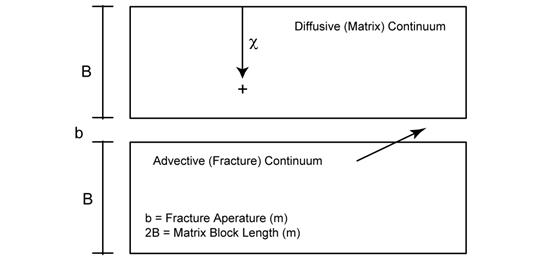
Figure PA- 30. Parallel-Plate, Dual-Porosity Conceptualization

PA-4.9.1.1 Advective Transport in Fractures

The PDE system used to represent advective transport in fractures is given by (WIPP Performance Assessment 1997b)

Ñ × (PA.268)

for k = 1, 2, ¼, nR, where

nR = number of radionuclides under consideration

C _k = concentration of radionuclide k in brine (kg/m³)

D k = hydrodynamic dispersion tensor (m²/s)

= Darcy velocity (i.e., specific discharge) of brine (m/s = (m³/m²)/s)

f = advective (i.e., fracture) porosity (dimensionless)

R _k = advective retardation coefficient (dimensionless)

l _k = decay constant for radionuclide k (s^- ¹)

Q _k = injection rate of radionuclide k per unit bulk volume of formation ((kg/s)/m³) (Note: Q k > 0 corresponds to injection into the fractures)

= mass transfer rate of radionuclide k per unit bulk volume of formation due to diffusion between fractures and surrounding matrix ((kg/s)/m³) (Note: > 0 corresponds to diffusion into fractures)

The Darcy velocity v is obtained from the solution of Equation (PA.263); specifically, v is defined by the relationship in Equation (PA.266). The advective porosity f , defined as the ratio of the interconnected fracture pore volume to the total volume, is determined by an uncertain parameter (see CFRCPOR in Table PA-17).

The hydrodynamic dispersion tensor is defined by (WIPP Performance Assessment 1997b; Bear 1972)

(PA.269)

where a _L and a _T are the longitudinal and transverse dispersivities (m); u and v are the x and y components of (i.e., v = [u, v]); is the free water molecular diffusion coefficient (m² s^- ¹) for radionuclide k; and t is the advective tortuosity, defined as the ratio of the true length of the flow path of a fluid particle to the straight-line distance between the starting and finishing points of the particle's motion. As in the CCA PA (Helton et al. 1998), the CRA-2014 PA uses a _L = a _T = 0 m and t = 1. Thus, the definition of D _k used in PA reduces to

(PA.270)

The diffusion coefficients, D*k, for the oxidation states of the radionuclides under consideration are shown in Table PA-14 (see parameters PU+3:MD0, PU+4:MD0, and U+6:MD0 in Kicker and Herrick 2013, Table 27). The existence of Pu in the (III) or (IV) oxidation state (i.e., as Pu(III) or Pu(IV)) and the existence of U in the (IV) or (VI) oxidation state (i.e., as U(IV) or U(VI)) is determined by an uncertain parameter (see WOXSTAT in Table PA-17).

Table PA- 14. Radionuclide Culebra Transport Diffusion Coefficients

Oxidation State	III	IV	VI
Diffusion Coefficient (m²/s)	3.00 ´ 10^-10	1.53 ´ 10^-10	4.26 ´ 10^-10

The advective retardation coefficient R _k is defined by

(PA.271)

where

r A = surface area density of fractures in Culebra (m²/m³ = 1/m) (i.e., surface area of fractures (m²) divided by volume of fractures (m³))

K Ak = surface area distribution coefficient ((kg/m²)/(kg/m³) = m) (i.e., concentration of radionuclide k sorbed on fracture surfaces (kg/m²) divided by concentration of radionuclide k dissolved in brine within fractures (kg/m³))

Following the logic used in the CCA (Helton et al. 1998), K _Ak = 0 and thus R _k = 1 are used in the PA.

In concept, the term Q _k in Equation (PA.268) provides the link between the releases to the Culebra calculated with NUTS and PANEL (Section PA-6.7) and transport within the Culebra. In the computational implementation of PA, radionuclide transport calculations in the Culebra were performed for unit radionuclide releases to the Culebra, and the outcomes of these calculations were used to construct the release to the accessible environment associated with time-dependent releases into the Culebra derived from NUTS and PANEL calculations (Section PA-6.8.3). The definition of Q _k is discussed in more detail in Section PA-4.9.1.4.

The initial condition for Equation (PA.268) is

kg/m³ (PA.272)

Furthermore, the boundary value conditions for Equation (PA.268) are defined at individual points on the boundary of the grid in Figure PA-28 on the basis of whether the flow vector v = [u, v] defines a flow entering the grid or leaving the grid. The following Neumann boundary value condition is imposed at points (x, y) where flow leaves the grid:

(PA.273)

where n(x, y) is an outward-pointing unit normal vector defined at (x, y). The following Dirichlet boundary value condition is imposed at points (x, y) where flow enters the grid:

kg/m³ (PA.274)

PA-4.9.1.2 Diffusive Transport in the Matrix

The system of PDEs used to represent diffusive transport in the matrix surrounding the fractures is given by (WIPP Performance Assessment 1997b)

(PA.275)

where χ is the spatial coordinate in Figure PA-30, is the matrix diffusion coefficient (m²/s) for radionuclide k defined by , and is the matrix tortuosity. The remaining terms have the same meaning as those in Equation (PA.268), except that the prime denotes properties of the matrix surrounding the fractures. A constant value ( ) for the matrix (i.e., diffusive) tortuosity is used in PA (Meigs 1996). The matrix (i.e., diffusive) porosity is an uncertain input to the analysis (see CMTRXPOR in Table PA-17). The matrix retardation is defined by

(PA.276)

where r _s is the particle density (kg/m³) of the matrix and K _dk is the distribution coefficient ((Ci/kg)/(Ci/m³) = m³/kg) for radionuclide k in the matrix. The density r _s is assigned a value of 2.82 ´ 10³ kg/m³ (Martell 1996b). The distribution coefficients K _dk are uncertain inputs to the analysis and dependent on the uncertain oxidation state of the relevant element (see CMKDAM3, CMKDPU3, CMKDPU4, CMKDTH4, CMKDU4, CMKDU6, and WOXSTAT in Table PA-17).

The initial and boundary value conditions used in the formulation of Equation (PA.275) are

(PA.277)

(PA.278)

(PA.279)

where (x, y) corresponds to a point in the domain on which Equation (PA.268) is solved and B is the matrix half-block length (m) in Figure PA-30 (i.e., 2B is the thickness of the matrix between two fractures). The initial condition in Equation (PA.277) means that no radionuclide is present in the matrix at the beginning of the calculation. The boundary value condition in Equation (PA.278) implies that no radionuclide movement can take place across the centerline of a matrix block separating two fractures. The boundary value condition in Equation (PA.279) ensures that the dissolved radionuclide concentration in the matrix at the boundary with the fracture is the same as the dissolved radionuclide concentration within the fracture. The matrix half-block length B is an uncertain input to the analysis (see CFRACSP in Table PA-17).

PA-4.9.1.3 Coupling Between Fracture and Matrix Equations

The linkage between Equation (PA.268) and Equation (PA.275) is accomplished through the term G _k , defining the rate at which radionuclide k diffuses across the boundary between a fracture and the adjacent matrix (see Figure PA-30). Specifically,

(PA.280)

where b is the fracture aperture (m) defined by

(PA.281)

PA-4.9.1.4 Source Term

As already indicated, Equation (PA.268) and Equation (PA.275) are solved for unit radionuclide releases to the Culebra. Specifically, a release of 1 kg of each of the four lumped radionuclides (²⁴¹Am, ²³⁴U, ²³⁰Th, and ²³⁹Pu) under consideration was assumed to take place over a time interval from 0 to 50 years, with this release taking place into the computational cell WPAC, located at the center of the Waste Panel Area in Figure PA-28, that has dimensions of 50 m ´ 50 m. The volume of this cell is given by

(PA.282)

where 4 m is the effective thickness of the Culebra Dolomite (Meigs and McCord 1996). As a result, Q _k (x, y, t) has the form

(PA.283)

for 0 £ t £ 50 yr and (x, y) in cell WPAC, and Q _k (x, y, t) = 0 (kg/m³/s) otherwise.

PA-4.9.1.5 Cumulative Releases

If denotes an arbitrary boundary (e.g., the LWB) in the domain of Equation (PA.268) (i.e., Figure PA-28), then the cumulative transport of C _k (t, B) of radionuclide k from time 0 to time t across is given by

(PA.284)

where h is the thickness of the Culebra (4 m), f is the advective porosity in Equation (PA.268), n(x, y) is an outward pointing unit normal vector, and denotes a line integral over B.

PA-4.9.2 Numerical Solution

The numerical solution to the coupled PDE system represented by Equation (PA.268) and Equation (PA.275) is computed using SECOTP2D, an implicit finite-volume code for the simulation of multispecies reactive transport. A high-level description of the numerical procedures implemented in SECOTP2D follows, with more detail available in WIPP Performance Assessment (1997b).

PA-4.9.2.1 Discretization of Fracture Domain

The fracture domain is discretized in space using the block-centered finite-difference method indicated in Figure PA-31. In this formulation, cell concentrations are defined at grid block centers while the velocity components [u, v] are defined on grid cell faces. A uniform mesh with 50 m ´ 50 m cells is used for the spatial discretization. Ghost cells are placed outside the problem domain for the purpose of implementing boundary conditions. The temporal discretization is accomplished using variable time step sizes.

Figure PA- 31. Schematic of Finite-Volume Staggered Mesh Showing Internal and Ghost Cells

The dispersive term,Ñ ×( fD _k Ñ C _k ), in Equation (PA.268) is approximated using a second-order central difference formula (Fletcher 1988).

The advective term , Ñ × v C _k , is approximated using the Total Variation Diminishing (TVD) method (Sweby 1984). The TVD method provides a way of accurately resolving advection-dominated transport problems without the occurrence of nonphysical oscillations commonly present in second-order solutions. This method invokes a weighted upstream differencing scheme that locally adjusts the weighting to prevent oscillatory behavior and maximize solution accuracy. The weighting parameters are known as the TVD flux limiters F(x, y, r), where r is a function of the concentration gradient and direction of flow. PA uses the van Leer TVD limiter (Sweby 1984, p. 1005), which is defined as

(PA.285)

At locations where u (i.e., the Darcy velocity in the x direction) is positive, r is defined at the
j -1/2, k interface by

(PA.286)

and at locations where u is negative, r is defined by

(PA.287)

Similar definitions are made for r at the j, k -1/2 interface in the y-direction with (i.e., the Darcy velocity in the y direction) used instead of u.

Because F _k is a function of C _k , the discretized set of equations is nonlinear. This nonlinearity is addressed by treating the flux limiters explicitly (i.e., time lagged). Explicit treatment of the limiter functions, however, can lead to oscillatory and sometimes unstable solutions when the Courant number exceeds unity (Cr > 1), where Cr is defined by

(PA.288)

To avoid this behavior, the application of the TVD method is restricted to regions in which the Courant numbers are less than one. In regions where Cr > 1, a first-order full upwinding scheme is invoked, which is unconditionally stable and nonoscillatory.

The discretized form of Equation (PA.268) can be expressed in a delta formulation as

(PA.289)

where is the identity matrix, L _xx and L _yy are finite-difference operators in the x and y directions, is an implicit source term that accounts for decay and mass transfer between the matrix and the fracture, RHS consists of the right-hand-side known values at time level n, and D C _n +1 = C _n +1 - C _n . Direct inversion of Equation (PA.289) for a typical Culebra transport problem is very computationally intensive, requiring large amounts of memory and time. To reduce these requirements, the operator in Equation (PA.289) is factored as follows:

(PA.290)

where a _x and a _y are constants that must sum to one (i.e., a _x + a _y = 1). The left-hand sides in Equation (PA.289) and Equation (PA.290) are not equivalent, with the result that the factorization of Equation (PA.289) and Equation (PA.290) is referred to as an approximate factorization (Fletcher 1988). The advantage of approximately factoring Equation (PA.289) is that the resulting equation consists of the product of two finite-difference operators that are easily inverted independently using a tridiagonal solver. Hence, the solution to the original problem is obtained by solving a sequence of problems in the following order:

(PA.291)

(PA.292)

(PA.293)

PA-4.9.2.2 Discretization of Matrix Equation

The nonuniform mesh used to discretize the matrix equation is shown in Figure PA-32. Straightforward application of standard finite-difference or finite-volume discretizations on nonuniform meshes results in truncation error terms that are proportional to the mesh spacing variation (Hirsch 1988). For nonuniform meshes, the discretization can be performed after a transformation from the Cartesian physical space (χ) to a stretched Cartesian computational space (ξ). The transformation is chosen so that the nonuniform grid spacing in physical space is transformed to a uniform spacing of unit length in computational space (the computational space is thus a one-dimensional domain with a uniform mesh). The transformed equations contain metric coefficients that must be discretized, introducing the mesh size influence into the difference formulas. Standard unweighted differencing schemes can then be applied to the governing equations in the computational space.

Figure PA- 32. Illustration of Stretched Grid Used for Matrix Domain Discretization

The SECOTP2D code applies such a coordinate transformation to the nonuniform diffusion domain mesh, solving the transformed system of equations in the uniform computational space. The transformed matrix equation is written as

(PA.294)

where

(PA.295)

(PA.296)

In the uniform computational space, a first-order backwards difference formula is used to approximate the temporal derivative, while a second-order accurate central difference is used to approximate spatial derivatives.

PA-4.9.2.3 Fracture-Matrix Coupling

The equations for the fracture and the matrix are coupled through the mass transfer term, G _k . In the numerical solution, these equations are coupled in a fully implicit manner and solved simultaneously. A procedure outlined in Huyakorn, Lester, and Mercer (1983) was adapted and redeveloped for an approximate factorization algorithm with the delta formulation and a finite-volume grid. The coupling procedure consists of three steps:

Step 1. Write the mass transfer term G _k in a delta ( ) form.

Step 2. Evaluate terms that are added to the implicit part of the fracture equation. This is accomplished using the inversion process (LU factorization) in the solution of the matrix equation. After the construction of the lower tridiagonal matrix L and the intermediate solution, there is enough information to evaluate the D terms. This new information is fed into the fracture equation that is subsequently solved for concentrations in the fracture at the new time level (n+1).

Step 3. Construct the boundary condition for the matrix equation at the fracture-matrix interface using fracture concentrations at the (n+1) time level. Matrix concentrations are then obtained using the upper tridiagonal matrix U by back substitution. A detailed description of this technique and its implementation is given in the SECOTP2D user's manual (WIPP Performance Assessment 1997b).

PA-4.9.2.4 Cumulative Releases

The cumulative transport C _k (t, B) of individual radionuclides across specified boundaries indicated in Equation (PA.284) is also accumulated during the numerical solution of Equation (PA.268) and Equation (PA.275).

PA-4.9.3 Additional Information

Because neither the Culebra flow fields nor the random seed used in LHS sampling have been changed from the CRA-2009 PABC, the radionuclide transport calculations from the CRA-2009 PABC were used in the CRA-2014 PA. Additional information on SECOTP2D and its use to determine radionuclide transport in the Culebra can be found in the SECOTP2D user's manual (WIPP Performance Assessment 1997b) and in the CRA-2009 PABC analysis package for radionuclide transport in the Culebra Dolomite (Kuhlman 2010).

PA-5.0 Probabilistic Characterization of Subjective Uncertainty

This section summarizes the treatment of uncertainty in the CRA-2014 PA parameters. This uncertainty gives rise to the epistemic uncertainty in the CCDFs defined in Section PA-2.2.4.

PA-5.1 Probability Space

As discussed in Section PA-2.2.4, the statement of confidence in the CCDFs of releases from the CRA-2014 PA is based on a probabilistic characterization of the uncertainty in important input parameters to the analysis. The probability distribution for each parameter is based on all available knowledge about the parameter, including measurements, and describes a degree of belief as to the appropriate range of the parameter value. This degree of belief depends on the numerical, spatial, and temporal resolution of the models selected for use in PA (Section PA-4.0). Correlations and other dependencies between imprecisely known variables are also possible. These relationships represent observed or logical dependencies between the possible parameter values.

The probability space that characterizes epistemic uncertainty can be represented as ( _su , _su , p _su ). The subscript su indicates that epistemic (i.e., subjective) uncertainty is being considered. The individual elements of _su are vectors v _su of the form

(PA.297)

where each v _j is an imprecisely known input to the analysis, and nv is the number of such inputs.

The uncertainty in the v _j , and hence in v _su , is characterized by developing a distribution

(PA.298)

for each v _j . It is the distributions in Equation (PA.297) and any associated correlations between the v _j that define ( _su , _su , p _su ).

The uncertain parameters incorporated into the CRA-2014 PA are discussed in Section PA-5.2, and the distributions and correlations assigned to these variables are described in Section PA-6.4 and Kicker and Herrick (Kicker and Herrick 2013), Table 4. Finally, a discussion of the concept of a scenario is given in Section PA-5.3.

PA-5.2 Variables Included for Subjective Uncertainty

The CRA-2014 PA identified 63 imprecisely known variables for inclusion in the analysis (see Kicker and Herrick 2013, Table 4). Most of the uncertain variables in the CRA-2014 PA were also treated as uncertain in the CRA-2009 PA. Most uncertain parameter additions and removals in the CRA-2014 PA relative to the CRA-2009 PA are due to the replacement of the Option D panel closure system with the ROMPCS and the refinement to the water budget implementation that includes MgO hydration. Table PA-15 and Table PA-16 list the additions and removals between the sets of uncertain parameters in the CRA-2009 PA and the CRA-2014 PA. All subjectively uncertain variables incorporated into the CRA-2014 PA are used as input to the models discussed in Section PA-2.2.3 and Section PA-4.0.

Table PA- 15. Sampled Parameters Added Since the CRA-2009 PA

Material	Property	Description
PCS_T1	PRMX_LOG	log₁₀ of intrinsic permeability, X direction
PCS_T1	SAT_RGAS	Residual gas saturation
PCS_T1	SAT_RBRN	Residual brine saturation
PCS_T1	PORE_DIS	Brooks-Corey pore distribution parameter
PCS_T1	POROSITY	Porosity
PCS_T2	POROSITY	Porosity
PCS_T2	POR2PERM	Quantity used to calculate intrinsic permeability using sampled porosity values
PCS_T3	POROSITY	Porosity
WAS_AREA	BRUCITEC	MgO inundated hydration rate in ERDA-6 brine
WAS_AREA	BRUCITES	MgO inundated hydration rate in Generic Weep Brine (GWB)
WAS_AREA	BRUCITEH	MgO humid hydration rate
WAS_AREA	HYMAGCON	Rate of conversion of hydromagnesite to magnesite

Table PA- 16. Sampled Parameters Removed Since the CRA-2009 PA

Material	Property	Description
CELLULS	FBETA	Factor beta for microbial reaction rates
CONC_PCS	PRMX_LOG	log₁₀ of intrinsic permeability, X direction
CONC_PCS	SAT_RGAS	Residual gas saturation
CONC_PCS	SAT_RBRN	Residual brine saturation
CONC_PCS	PORE_DIS	Brooks-Corey pore distribution parameter

Each uncertain variable is assigned a distribution that characterizes the subjective uncertainty in that variable. Distributions for each parameter are described in Kicker and Herrick (Kicker and Herrick 2013) Table 4, which also contains documentation for each of the 63 parameters sampled by the LHS code during the PA. The set of subjectively uncertain variables are listed in Table PA-17. The input files used for PA code STEPWISE use short names for input parameters rather than material:property designations used in other codes. These short names are required because of a limitation in the length of variable names in STEPWISE. The short names used in STEPWISE are listed in Table PA-17 under the "Name" column, and are taken from Table 1 of Kirchner (2013b).

Table PA- 17. Variables Representing Epistemic Uncertainty in the CRA-2014 PA

Material	Property	Name	Description
AM+3	MKD_AM	CMKDAM3	Matrix distribution coefficient (m³/kg) for Am in the III oxidation state. Defines K _dk in Equation (PA.276).
BH_SAND	PRMX_LOG	BHPERM	Logarithm of intrinsic permeability (m²) of the silty-sand-filled borehole (Table PA-7). Used in regions Upper Borehole and Lower Borehole in Figure PA-12.
BOREHOLE	DOMEGA	DOMEGA	Drill string angular velocity (rad/s). Defines in Equation (PA.139 ).
BOREHOLE	TAUFAIL	WTAUFAIL	Shear strength of waste (Pa). Defines t (R, 1) in Equation (PA.137).
CASTILER	COMP_RCK	BPCOMP	Bulk compressibility (Pa^-1) of Castile brine reservoir. Defines c _fB in Equation (PA.35) for region CASTILER of Figure PA-12.
CASTILER	PRESSURE	BPINTPRS	Initial brine pore pressure in the Castile brine reservoir (region CASTILER in Figure PA-12).
CASTILER	PRMX_LOG	BPPRM	Logarithm of intrinsic permeability (m²) of the Castile brine reservoir. Used in region CASTILER in Figure PA-12.
CONC_PLG	PRMX_LOG	PLGPRM	Logarithm of intrinsic permeability (m²) of the concrete borehole plugs (Table PA-7). Used in region Borehole Plugs in Figure PA-12.
CULEBRA	APOROS	CFRACPOR	Culebra fracture (i.e., advective) porosity (dimensionless). Defines f in Equation (PA.268).
CULEBRA	DPOROS	CMTRXPOR	Culebra matrix (i.e., diffusive) porosity (dimensionless). Defines f' in Equation (PA.275).
CULEBRA	HMBLKLT	CFRACSP	Culebra fracture spacing (m). Equal to half the distance between fractures (i.e., the Culebra half-matrix-block length).
CULEBRA	MINP_FAC	CTRANSFM	Multiplier (dimensionless) applied to transmissivity of the Culebra within the LWB after mining of potash reserves. Defines MF in Equation (PA.261) (see Section PA-4.8.2).
DRZ_1	PRMX_LOG	DRZPRM	Logarithm of intrinsic permeability (m²) of the DRZ. Used in regions Upper DRZ and Lower DRZ in Figure PA-12.
DRZ_PCS	PRMX_LOG	DRZPCPRM	Logarithm of intrinsic permeability (m²) of the DRZ immediately above and below the panel closure (Section PA-4.2.8). Used in region DRZ_PCS in Figure PA-12.
GLOBAL	CLIMTIDX	CCLIMSF	Climate scale factor (dimensionless) for Culebra flow field. Defines SFC in Equation (PA.266).
GLOBAL	OXSTAT	WOXSTAT	Indicator variable for elemental oxidation states (dimensionless). WOXSTAT <= 0.5 indicates radionuclides in lower oxidation states. WOXSTAT >0.5 indicates radionuclides in higher oxidation states.

Table PA-17. Variables Representing Epistemic Uncertainty in the CRA-2014 PA (Continued)
Material	Property	Name	Description
GLOBAL	PBRINE	PBRINE	Probability that a drilling intrusion penetrates pressurized brine in the Castile. Defines pB ₁; see Section PA-3.6.
GLOBAL	TRANSIDX	CTRAN	Indicator variable for selecting T-field. See Section PA-4.8.2.
PCS_T1	PORE_DIS	T1PDIS	Brooks-Corey pore distribution parameter
PCS_T1	POROSITY	T1POROS	Effective porosity
PCS_T1	PRMX_LOG	T1PRMX	Log of intrinsic permeability, X-direction
PCS_T1	SAT_RBRN	T1SRBRN	Residual Brine Saturation
PCS_T1	SAT_RGAS	T1SRGAS	Residual Gas Saturation
PCS_T2	POR2PERM	T2P2PERM	Distribution used to calculate permeability from sampled porosity values
PCS_T2	POROSITY	T2POROS	Effective porosity
PCS_T3	POROSITY	T3POROS	Effective porosity
PHUMOX3	PHUMCIM	WPHUMOX3	Ratio (dimensionless) of concentration of actinides attached to humic colloids to dissolved concentration of actinides for oxidation state III in Castile brine.
PU+3	MKD_PU	CMKDPU3	Matrix distribution coefficient (m³/kg) for Pu in III oxidation state. Defines K_dk in Equation (PA.276 ).
PU+4	MKD_PU	CMKDPU4	Matrix distribution coefficient (m³/kg) for Pu in IV oxidation state. Defines K_dk in Equation (PA.276 ).
S_HALITE	COMP_RCK	HALCROCK (previously HALCOMP)	Bulk compressibility of halite (Pa^-1). Defines c _r in Equation (PA.37) for Salado region of Figure PA-12.
S_HALITE	POROSITY	HALPOR	Halite porosity (dimensionless). Defines f ₀ in Equation (PA.30) for Salado region in Figure PA-12.
S_HALITE	PRESSURE	SALPRES	Initial brine pore pressure (Pa) in the Salado halite, applied at an elevation consistent with the intersection of MB 139. Defines p_b,ref for Equation (PA.53) for Salado region in Figure PA-12.
S_HALITE	PRMX_LOG	HALPRM	Logarithm of intrinsic halite permeability (m²). Used in region Salado in Figure PA-12.
S_MB139	PORE_DIS	ANHBCEXP	Brooks-Corey pore distribution parameter for anhydrite (dimensionless). Defines l in Equation (PA.38), Equation (PA.39), and Equation (PA.40) for regions MB 138, Anhydrite AB, and MB 139 of Figure PA-12 for use with Brooks-Corey model; defines l in m = l /(1 + l ) in Equation (PA.44), Equation (PA.45), and Equation (PA.46) for use with van Genuchten-Parker model in the same regions.
S_MB139	PRMX_LOG	ANHPRM	Logarithm of intrinsic anhydrite permeability (m²). Used in regions MB 138, Anhydrite AB, and MB 139 in Figure PA-12.
S_MB139	RELP_MOD	ANHBCVGP	Indicator for relative permeability model (dimensionless) for regions MB 138, Anhydrite AB, and MB 139 in Figure PA-12. See Table PA-4.
S_MB139	SAT_RBRN	ANRBRSAT	Residual brine saturation in anhydrite (dimensionless). Defines S_br in Equation (PA.43) for regions MB 138, Anhydrite AB, and MB 139 in Figure PA-12.
SHFTL_T1	PRMX_LOG	SHLPRM2	Logarithm of intrinsic permeability (m²) of lower shaft-seal materials for the first 200 years after closure. Used in Lower Shaft region in Figure PA-12.
SHFTL_T2	PRMX_LOG	SHLPRM3	Logarithm of intrinsic permeability (m²) of lower shaft-seal materials from 200 years to 10,000 years after closure. Used in Lower Shaft region in Figure PA-12.
SHFTU	PRMX_LOG	SHUPRM	Logarithm of intrinsic permeability (m²) of upper shaft-seal materials. Used in Upper Shaft region in Figure PA-12.
SHFTU	SAT_RBRN	SHURBRN	Residual brine saturation in upper shaft-seal materials (dimensionless). Defines S _br in Equation (PA.43) for Upper Shaft region in Figure PA-12.
SHFTU	SAT_RGAS	SHURGAS	Residual gas saturation in upper shaft-seal materials (dimensionless). Defines S_gr in Equation (PA.42) for Upper Shaft region in Figure PA-12.
SOLMOD3	SOLVAR	WSOLVAR3	Solubility multiplier (dimensionless) for III oxidation states. Used by ALGEBRA prior to PANEL (Section PA-4.4, Brush and Domski 2013c).
SOLMOD4	SOLVAR	WSOLVAR4	Solubility multiplier (dimensionless) for IV oxidation states. Used by ALGEBRA prior to PANEL (Section PA-4.4, Brush and Domski 2013c).
SPALLMOD	PARTDIAM	SPPDIAM (previously SPLPTDIA, WPRTDIAM)	Particle diameter of waste (m) after tensile failure, implemented by parameter SPALLMOD/PARTDIAM. Loguniform distribution from 0.001 to 0.1 (m). Defines d_p in Equation (PA.192 ).
SPALLMOD	REPIPERM	REPIPERM	Waste permeability of gas (m²) local to intrusion borehole. Defines k in Equation (PA.174).
SPALLMOD	REPIPOR	SPLRPOR	Waste porosity (dimensionless) at time of drilling intrusion. Defines f in Equation (PA.173).
SPALLMOD	TENSLSTR	TENSLSTR	Tensile strength (Pa) of waste. Defines in Section PA-4.6.2.3.4.
STEEL	CORRMCO2	WGRCOR	Rate of anoxic steel corrosion (m/s) under brine-inundated conditions with no CO₂ present. Defines R_ci in Equation (PA.67) for areas Waste Panel, South RoR, and North RoR in Figure PA-12.
TH(IV)	MKD_TH	CMKDTH4	Matrix distribution coefficient (m³/kg) for Th in IV oxidation state. Defines K_dk in Equation (PA.276 ).
U(IV)	MKD_U	CMKDU4	Matrix distribution coefficient (m³/kg) for U in IV oxidation state. Defines K_dk in Equation (PA.276 ).
U(VI)	MKD_U	CMKDU6	Matrix distribution coefficient (m³/kg) for U in VI oxidation state. Defines K_dk in Equation (PA.276 ).
WAS_AREA	BIOGENFC	WBIOGENF	Probability of obtaining sampled microbial gas generation rates.
WAS_AREA	BRUCITEC	WBRUITEC	Waste emplacement area and waste,MgO inundated hydration rate in ERDA-6 brine
WAS_AREA	BRUCITEH	WBRUITEH	Waste emplacement area and waste,MgO humid hydration rate
WAS_AREA	BRUCITES	WBRUITES	Waste emplacement area and waste,MgO inundated hydration rate in GWB
WAS_AREA	GRATMICH	WGRMICH	Rate of CPR biodegradation (mol C₆H₁₀O₅ / kg C₆H₁₀O₅ /s) under anaerobic, humid conditions.
WAS_AREA	GRATMICI	WGRMICI	Rate of CPR biodegradation (mol C₆H₁₀O₅ / kg C₆H₁₀O₅ /s) under anaerobic, brine-inundated conditions.
WAS_AREA	HYMAGCON	WHYMAGC	Waste emplacement area rate of conversion of hydromagnesite to magnesite
WAS_AREA	PROBDEG	WMICDFLG	Index for model of CPR material microbial degradation (dimensionless). Used in Waste Panel, South RoR, and North RoR areas in Figure PA-12.
WAS_AREA	SAT_RBRN	WRBRNSAT	Residual brine saturation in waste (dimensionless). Defines S _br in Equation (PA.42) for Waste Panel, South RoR, and North RoR areas in Figure PA-12; also used in waste material in Figure PA-24 for DBR calculation; see Section PA-4.7.
WAS_AREA	SAT_RGAS	WRGSSAT	Residual gas saturation in waste (dimensionless). Defines S_gr in Equation (PA.43) for Waste Panel, South RoR, and North RoR areas in Figure PA-12; also used in waste material in Figure PA-24 for DBR calculation; see Section PA-4.7.
WAS_AREA	SAT_WICK	WASTWICK	Increase in brine saturation of waste due to capillary forces (dimensionless). Defines S_wick in Equation (PA.99) for Waste Panel, South RoR, and North RoR areas in Figure PA-12.

PA-5.3 Separation of Aleatory and Epistemic Uncertainty

PA uses the term scenario to refer to specific types of events within the sample space for aleatory uncertainty (E0, E1, E2, or E1E2; see Section PA-3.10). This definition is consistent with the concept that a scenario is something that could happen in the future. A future contains events of the form defined in Equation (PA.2) and is associated with a probability, one that characterizes the likelihood that a possible future will match the occurrences that will take place at the WIPP over the next 10,000 years. In contrast, the probability associated with a specific vector v _su , i.e., a specific set of parameter values, characterizes a degree of belief that the vector contains the appropriate values for the 63 uncertain variables in CRA-2014 PA. The distribution of epistemic vectors defines the impact of parameter uncertainty over the full range of possible futures and is used to establish confidence in the results.

PA-6.0 Computational Procedures

This section outlines the computational procedures used to execute the CRA-2014 PA. First, the sampling procedures applied to evaluate performance accounting for epistemic and aleatory uncertainty are outlined. The mechanistic calculations used to evaluate the function f(x _st ) in Equation (PA.23) are tabulated, followed by a description of the algorithms used to compute releases. This section concludes with a discussion of sensitivity analysis techniques used to identify which uncertain parameters are primary contributors to the uncertainty in the PA results.

PA-6.1 Sampling Procedures

Extensive use is made of sampling procedures in PA. In particular, simple random sampling is used to generate individual CCDFs (Section PA-2.2.3) and LHS is used to assess the effects of imprecisely known model parameters (Section PA-2.2.4).

Using simple random sampling, a possible future, x _st,i,k , is characterized by the collection of intrusion events occurring in that future (see Section PA-2.2.2). The subscript st denotes that intrusion is modeled as a stochastic (or random) process, the subscript i indicates that the future is one of many possible futures, and the subscript k indicates that the vector of uncertain parameter sampled values is one of many such vectors. The nR sets of values (possible futures) are selected according to the joint probability distribution for the elements of _st as defined by ( _st , _st , p _st ). In practice, the joint probability distribution is defined by specifying a distribution D _j for each element x _j of _st . Points from different regions of the sample space occur in direct relationship to the probability of occurrence of these regions. Furthermore, each sample element is selected independently of all other sample elements. The values selected using simple random sampling provide unbiased estimates for means, variances, and distributions of the variables. The collection of nR samples can be denoted as a vector x _st,k :

(PA.299)

The WIPP PA code CCDFGF is used to simulate possible futures based on the values of the variables sampled. These variables control the stochastic processes defined within CCDFGF, such as the time when a drilling intrusion can take place, where that drilling intrusion is located, and whether the drilling intrusion encounters an excavated area. The code CCDFGF is capable of generating and evaluating thousands of possible futures; PA uses a sample size (nR) of 10,000 to generate a distribution of possible repository releases. This sample size is sufficient to estimate the 0.999 quantile for the distribution of releases to the accessible environment.

LHS is used to sample the parameters for which distributions of epistemic uncertainty were defined to integrate over the probability space for subjective uncertainty ( _su , _su , p _su ). This technique was first introduced by McKay, Beckman, and Conover (1979). In LHS, the range of each uncertain parameter v _j is divided into nLHS intervals of equal probability and one value is selected at random from each interval. The nLHS values thus obtained for v ₁ are paired at random without replacement with the nLHS values obtained for v ₂. These nLHS pairs are combined in a random manner without replacement with the nLHS values of v ₃ to form nLHS triples. This process is continued until a set of nLHS nV-tuples is formed. These nV-tuples are of the form

, k = 1, ..., nLHS (PA.300)

and constitute the Latin hypercube sample. The individual v _j s must be independent of each other for the preceding construction procedure to work. For more information about LHS and a comparison with other sampling techniques, see Helton and Davis (Helton and Davis 2003).

LHS stratifies the sampling to ensure that the sampled values cover the full range of each v _j in the nLHS samples. LHS provides unbiased estimates for means and distribution functions of each sampled variable (McKay, Beckman, and Conover 1979). In particular, uncertainty and sensitivity analysis results obtained with LHS are robust even when relatively small samples (i.e., nLHS = 50 to 200) are used (Iman and Helton 1988 and Iman and Helton 1991; Helton et al. 1995).

When sampling for both aleatory uncertainty and epistemic uncertainty are considered, the joint sample space, x, consists of a vector of nLHS vectors of possible futures:

(PA.301)

The differences between the nLHS futures are due to the uncertainty in the v _j , i.e. the epistemic uncertainty in model parameters.

PA-6.2 Sample Size for Incorporation of Subjective Uncertainty

Section 194.34(d) states that

The number of CCDFs generated shall be large enough such that, at cumulative releases of 1 and 10, the maximum CCDF generated exceeds the 99^th percentile of the population of CCDFs with at least a 0.95 probability.

For an LHS of size nLHS, the preceding guidance is equivalent to the inequality

(PA.302)

which results in a minimum value of 298 for nLHS. PA uses a total sample size of 300 to represent the epistemic uncertainty. As discussed in the next section, the 300 samples are divided among 3 replicates of size 100 each to demonstrate convergence of the mean for the population of CCDFs.

PA-6.3 Statistical Confidence on Mean CCDF

Section 194.34(f) states,

Any compliance assessment shall provide information which demonstrates that there is at least a 95% level of statistical confidence that the mean of the population of CCDFs meets the containment requirements of § 191.13 of this chapter.

Given that LHS is used, the confidence intervals required by section 194.34(f) are obtained with a replicated sampling technique proposed by Iman (Iman 1982). In this technique, the sampling in Equation (PA.303) is repeated nS times with different random seeds. These samples lead to a sequence r = 1, 2, …, nS of estimated mean exceedance probabilities, where defines the mean CCDF obtained for sample r (i.e., is the mean probability that a normalized release of size R will be exceeded; see Section PA-2.2.4) and nS is the number of independent samples generated with different random seeds. The seed of the random number generator determines the sequence of the numbers it generates. Then,

(PA.303)

and

(PA.304)

provide an additional estimate of the mean CCDF and an estimate of the standard error (SE(R)) associated with the mean exceedance probabilities. The t-distribution with nS -1 degrees of freedom can be used to place confidence intervals around the mean exceedance probabilities for individual R values (i.e., around ). Specifically, the 1- a confidence interval is given by , where is the quantile of the t-distribution with nS -1 degrees of freedom (e.g., for a = 0.05 and nS = 3). The same procedure can also be used to place pointwise confidence intervals around percentile curves. The mean and its standard error could equally well be computed from one replicate of size 300. However, the use of three replicates, each with its own random seed, minimizes the impact of any one seed used in random number generation. The three replicates have also been useful in evaluating the presence of spurious correlations among parameters and releases in the sensitivity analyses.

PA-6.4 Generation of Latin Hypercube Samples

The LHS program (WIPP Performance Assessment 2005) is used to produce three independently generated Latin hypercube samples of size nLHS = 100 each, for a total of 300 sample elements. Each individual replicate is a Latin hypercube sample of the form

, k = 1, 2, ¼, nLHS = 100 ( PA.305)

In the context of the replicated sampling procedure described in Section PA-6.2, nS = 3 replicates of 100 are used. For notational convenience, the replicates are designated by R1, R2, and R3.

The restricted pairing technique described in Section PA-6.1 is used to induce requested correlations and also to assure that uncorrelated variables have correlations close to zero. The variable pairs (S_HALITE:PRMX_LOG, S_HALITE:COMP_RCK) and (CASTILER:
PRMX_LOG, CASTILER:COMP_RCK) are assigned rank correlations of -0.99 and -0.75, respectively. All other variable pairs are assigned rank correlations of zero. The restricted pairing technique successfully produces these correlations (Table PA-18). Correlated variables have correlations that are close to their specified values.

Table PA- 18. Observed and Expected Correlations Between Variable Pairs (S_HALITE:COMP_RCK, S_HALITE:PRMX_LOG) and (CASTILER:COMP_RCK ,CASTILER:PRMX_LOG)

Replicate	Between		Expected Correlation	Observed Correlation
1	CASTILER:COMP_RCK	CASTILER:PRMX_LOG	-0.75	-0.7281
1	S_HALITE:COMP_RCK	S_HALITE:PRMX_LOG	-0.99	-0.9869
2	CASTILER:COMP_RCK	CASTILER:PRMX_LOG	-0.75	-0.7242
2	S_HALITE:COMP_RCK	S_HALITE:PRMX_LOG	-0.99	-0.9907
3	CASTILER:COMP_RCK	CASTILER:PRMX_LOG	-0.75	-0.7252
3	S_HALITE:COMP_RCK	S_HALITE:PRMX_LOG	-0.99	-0.9834

The code LHS_EDIT (Kirchner 2013a) was used to enforce a conditional relationship between three pairs of variables. The relationships were WAS_AREA:GRATMICH ≤ WAS_AREA:GRATMICI (Clayton 2008a, Nemer and Stein 2005) and PCS_T3: POROSITY ≤ PCS_T2: POROSITY ≤ PCS_T1:POROSITY (Camphouse 2013d). The relationships were enforced by modifying values in the LHS transfer file, thus making the conditioned values available for use in the sensitivity analysis. For each pair of variables LHS_EDIT rescales the sampled value of the parameter to the left of the ≤ symbol to the new "controlled" value using the equation

(PA.306)

where is the conditioned value of the left hand variable, v_i is the sampled value of that variable, x_i is the sampled value of the right hand variable, and U_V,lower and U_V,upper are the bounds of the distribution assigned to the left hand variable. This method preserves the probability associated with the value of the left hand variable.

PA-6.5 Generation of Individual Futures

Simple random sampling (Section PA-6.1) is used to generate 10,000 possible futures that are then used to construct CCDFs of potential releases. Table PA-19 outlines the algorithm used to generate a single future in PA.

Table PA- 19. Algorithm to Generate a Single Future

1. Sample t_i,1 with a time dependent l _d given by

where t _A = 100 yr (i.e., time at which administrative control ends) and l _d = 4.23 ´ 10^-3 yr^-1 (see Section PA-3.3). The index i is the number of the future and 1 represents the first intrusion event.

2. Sample e_i,1 with a probability of p[E0] = 0.797 that the intrusion will be in an unexcavated area and a probability of p[E1] = 0.203 that the intrusion will be in an excavated area (see Section PA-3.4).

3. Sample l_i,1 with a probability of p[L_j ] = 6.94 ´ 10^-3 for each of the j = 1, 2, ¼, 144 nodes in Figure PA-11 (see Section PA-3.5).

4. Sample b_i,1 with a probability of p[B ₁] that the intrusion will penetrate pressurized brine (see Section PA-3.6). p[B ₁] is sampled from a normal distribution ranging from 0.06 to 0.19.

5. Sample p _i,1 with probabilities of p[PL1] = 0.04, p[PL2] = 0.594, and p[PL3] = 0.366 that plugging pattern 1, 2, or 3, respectively, will be used (see Section PA-3.7).

6. Sample the activity level a _i,1 (see Section PA-3.8).

6.1 Penetration of nonexcavated area (i.e., e_i,1 = 0): a _i,1 = a_i,1 = 0.

6.2 Penetration of excavated area (i.e., e_i,1 = 1): Sample to determine if intrusion penetrates RH-TRU or CH- TRU waste with probabilities of p[RH] = 0.124 and p[CH] = 0.876 of penetrating RH-TRU and CH-TRU waste, respectively.

6.3 Penetration of RH-TRU waste: a _i,1 = a_i,1 = 1.

6.4 Penetration of CH-TRU waste: Use probabilities p[CH_j ] of intersecting waste stream j, j = 1, 2, ¼, 451, (see Kicker and Zeitler 2013a) to independently sample three intersected waste streams iCH11, iCH12, iCH13 (i.e., each of iCH11, iCH12, iCH13 is an integer between 1 and 451). Then, a _i,1 = [2, iCH11, iCH12, iCH13].

7. Repeat Steps 1 - 6 to determine properties (i.e., t_i,j, e_i,j, l_i,j, b_i,j, p_i,j, a _i,j ) of the j^th drilling intrusion.

8. Continue until t_n ₊₁ > 10,000 yr; the n intrusions thusly generated define the drilling intrusions associated with x _st,i .

9. Sample t_min with a time dependent l _m given by

where t_A = 100 yr and l _m = 1 ´ 10^-4 yr^-1 (see Section PA-3.9).

For each vector of the LHS sample, a total of nS = 10,000 individual futures of the form

(PA.307)

are generated in the construction of all CCDFs for that LHS vector. As 300 LHS vectors are used in the analysis and 10,000 futures are sampled for each LHS vector, the total number of futures used in the analysis for CCDF construction is 3 ´ 10⁶.

The drilling rate l _d is used to generate the times at which drilling intrusions occur. For a Poisson process with a constant l _d (i.e., a stationary process), the cumulative distribution function (CDF) for the time D t between the successive events is given by (Ross 1987, p. 113)

( PA.308)

A uniformly distributed random number r ₁ is selected from [0, 1]. Then, solution of

(PA.309)

for t ₁ gives the time of the first drilling intrusion. An initial period of 100 years of administrative control is assumed; thus 100 years is added to the t ₁ obtained in Equation (PA.309) to obtain the time of the first drilling intrusion. Selecting a second random number r ₂ and solving

(PA.310)

for D t ₁ gives the time interval between the first and second drilling intrusions, with the outcome that . This process continues until t _n ₊₁ exceeds 10,000 years. The times t ₁, t ₂, ¼, t _n then constitute the drilling times in that possible future..

The mining time t _min is sampled in a manner similar to the drilling times. Additional uniformly distributed random numbers from [0,1] are used to generate the elements e _j , l _j , b _j , p _j , a _j of x _st,i from their assigned distributions (see Section PA-2.2.2).

PA-6.6 Construction of CCDFs

In PA, the sampling of individual futures (Section PA-6.5) and associated CCDF construction is carried out by the CCDFGF program (WIPP Performance Assessment 2010). The sampled futures x _st,i in Equation (PA.307) are used to construct CCDFs for many different quantities (e.g., cuttings and cavings releases, spallings releases, DBRs, etc.). The construction process is the same for each quantity. For notational convenience, assume that the particular quantity under consideration can be represented by a function f (x _st,i ), with the result that 10,000 values

, i = 1, 2, ¼, 10,000 (PA.311)

are available for use in CCDF construction. Formally, the resultant CCDF is defined by the expression in Equation (PA.3). In practice, the desired CCDF is obtained after ordering f(x _st,i ) from smallest to largest or largest to smallest, as described below.

PA uses a binning procedure in CCDF construction to simplify sorting the individual f(x _st,i ) and to reduce the number of plot points. Specifically, the range of f(x _st,i ) is divided into intervals (i.e., bins) by the specified points

(PA.312)

where f _min is the minimum value of f(x _st,i ) to be plotted (typically 10^- ⁶ or 10^- ⁵ for an EPA-normalized release), f _max is the maximum value of f to be plotted (typically 100 for an EPA-normalized release), n is the number of bins in use, and the b _i are typically loguniformly distributed with 20 values per order of magnitude. A counter nB _j is used for each interval [b _j 1,b _j ]. All counters are initially set to zero. Then, as individual values f(x _st,i ) are generated, the counter nB _j is incremented by 1 when the inequality

(PA.313)

is satisfied. When necessary, f _max is increased in value so that the inequality f(x _st,i ) < fmax will always be satisfied. Once the 10,000 values for f(x _st,i ) have been generated, a value of nB _j exists for each interval [b _j -1, b _j ]. The quotient

(PA.314)

provides an approximation to the probability that f(x _st,i ) will have a value that falls in the interval [b _j -1, b _j ]. The resultant CCDF is then defined by the points

(PA.315)

for j = 0, 1, 2, ¼, n -1, where prob(value > b _j ) is the probability that a value greater than b _j will occur.

The binning technique produces histograms that are difficult to read when multiple CCDFs appear in a single plot. As the number of futures is increased and the bins are refined, the histogram CCDF should converge to a continuous CCDF as additional points are used in its construction. The continuous CCDF is approximated by drawing diagonal lines from the left end of one bin to the left end of the next bin.

When multiple CCDFs appear in a single plot, the bottom of the plot becomes very congested as the individual CCDFs drop to zero on the abscissa. For this reason, each CCDF stops at the largest observed consequence value among the 10,000 values calculated for that CCDF. Stopping at the largest consequence value, rather than the left bin boundary of the bin that contains this value, permits the CCDF to explicitly show the largest observed consequence. Because a sample size of 10,000 is used in the generation of CCDFs for comparison with the EPA release limits, the probability corresponding to the largest observed consequence is typically 10^- ⁴.

PA-6.7 Mechanistic Calculations

In the CRA-2014 PA, calculations were performed with the models described in Section PA-4.0 for selected elements of S _st (see Section PA-3.10), and the results were used to determine the releases to the accessible environment for the large number (i.e., 10,000) of randomly sampled futures used to estimate individual CCDFs. The same set of mechanistic calculations was performed for each LHS element. This section summarizes the calculations performed with each of the models described in Section PA-4.0; Section PA-6.8 outlines the algorithms used to construct releases for the randomly sampled elements x _st,i of S _st from the results of the mechanistic calculations. Long (2013) documents execution of the calculations and archiving of calculation results.

PA-6.7.1 BRAGFLO Calculations

The BRAGFLO code (Section PA-4.2) computes two-phase (brine and gas) flow in and around the repository. BRAGFLO results are used as initial conditions in the models for Salado transport (implemented in NUTS and PANEL), spallings (implemented in CUTTINGS_S), and DBR (also calculated by BRAGFLO). Thus, the BRAGFLO scenarios are used to define scenarios for other codes.

The four fundamental scenarios for the CRA-2014 PA (Section PA-3.10) define four categories of calculations to be performed with BRAGFLO (i.e., E0, E1, E2, and E1E2). These four fundamental scenarios were expanded into six general scenarios by specifying the time of drilling intrusions. Table PA-20 summarizes the specific scenarios used in the CRA-2014 PA. A total of 6 scenarios ´ nR ´ nLHS = 6 ´ 3 ´ 100 = 1,800 BRAGFLO calculations were conducted for the CRA-2014 PA.

Table PA- 20. BRAGFLO Scenarios in the CRA-2014 PA

Fundamental Scenario (Section PA-3.10)	Specific Scenario	Time of Drilling Intrusion(s)
E0: no drilling intrusions.	S1-BF	N/A
E1: single intrusion through an excavated area of the repository that penetrates pressurized brine in the Castile.	S2-BF	350 years
	S3-BF	1,000 years
E2: single intrusion through an excavated area of the repository that does not penetrate pressurized brine in the Castile.	S4-BF	350 years
	S5-BF	1,000 years
E1E2: two intrusions into the same waste panel, the first being an E2 intrusion and the second being an E1 intrusion.	S6-BF	1,000 years for E2 intrusion 2,000 years for E1 intrusion

Values for the activity level a ₁ and mining time t _min are not needed for the mechanistic calculations; these values are used in the construction of the releases from the results of the mechanistic calculations (Section PA-6.8). Although a value for drilling location l ₁ is not specified, a drilling location is required for the BRAGFLO calculations. If equivalent grids were used in the definition of x _st,i (Figure PA-11) and in the numerical solution of the PDEs on which BRAGFLO is based (Figure PA-12), the location of the drilling intrusion used in the BRAGFLO calculations could be specified as a specific value for l ₁, which in turn would correspond to one of the 144 locations in Figure PA-11 designated by l in the definition of x _st,i . However, as these grids are not the same, a unique pairing between a value for l ₁ and the location of the drilling intrusion used in the computational grid employed with BRAGFLO is not possible. The BRAGFLO computational grid divides the repository into a lower waste panel (Waste Panel area), a middle group of four waste panels (South RoR area), and an upper group of five waste panels (North RoR area), with the drilling intrusion taking place through the center of the lower panel (Figure PA-12). Thus, in the context of the locations in Figure PA-11 potentially indexed by l ₁, the drilling intrusions in Scenarios S2-S5 occur at a location in Panel 5, which is the southernmost panel. In Scenario S6, both intrusions occur at a location in Panel 5, with the effects of flow between the two boreholes implemented through assumptions involving the time-dependent behavior of borehole permeability (Table PA-7).

PA-6.7.2 NUTS Calculations

For Scenarios S1-BF to S5-BF, radionuclide transport through the Salado is computed by the code NUTS (Section PA-4.3) using the flow fields computed by BRAGFLO. Two types of calculations are performed with NUTS. First, a set of screening calculations identifies elements of the sample from _su for which radionuclide transport through the Salado to the LWB or Culebra is possible. The screening calculations identify a subset of the sample from _su for which transport is possible and for which release calculations are performed. Screening calculations are performed for BRAGFLO Scenarios S1-BF to S5-BF, for a total of 1,500 screening calculations with NUTS. For each vector that is retained (based on the screening calculations), release calculations are performed for a set of intrusion times.

Table PA-21 lists five scenarios for release calculations corresponding to the five BRAGFLO scenarios. Each NUTS scenario uses the flow field computed for the corresponding BRAGFLO scenario. The intrusion times for the NUTS scenarios are accommodated by shifting the BRAGFLO flow fields in time so that the NUTS and BRAGFLO intrusions coincide. For example, the NUTS S3 scenario with an intrusion at 3,000 years requires a flow field for the time interval between (3,000 years and 10,000 years); this scenario uses the BRAGFLO S3-BF scenario flow field for the time interval between (1,000 years and 8,000 years).

Table PA- 21. NUTS Release Calculations in the CRA-2014 PA

NUTS Scenario	Number of Vectors with Releases				Flow field	Intrusion Time ( t1)
NUTS Scenario	R1	R2	R3	Total	Flow field	Intrusion Time ( t1)
S1	0	0	0	0	BRAGFLO S1-BF scenario	N/A
S2	87	88	92	267	BRAGFLO S2-BF scenario	E1 intrusion at 100 and 350 years
S3	79	81	81	241	BRAGFLO S3-BF scenario	E1 intrusion at 1,000, 3,000, 5,000, 7,000, or 9,000 years
S4	19	22	20	61	BRAGFLO S4-BF scenario	E2 intrusion at 100 and 350 years
S5	17	22	16	55	BRAGFLO S5-BF scenario	E2 intrusion at 1,000, 3,000, 5,000, 7,000, or 9,000 years

Values for the variables indicating intrusion into an excavated area (e ₁), penetration of pressurized brine (b ₁), plugging pattern (p ₁), and drilling location (l ₁) are the same as in the corresponding BRAGFLO scenario. Values for the activity level a ₁ and mining time t _min are not specified for the NUTS scenarios.

PA-6.7.3 PANEL Calculations

As outlined in Section PA-4.4, the code PANEL is used to estimate releases to the Culebra associated with E1E2 scenarios and to estimate radionuclide concentrations in brine for use in estimating DBRs. An E1E2 scenario assumes two drilling intrusions into the same waste panel: the first an E2 intrusion (Table PA-20) occurring at time t ₁ and the second an E1 intrusion (Table PA-20) occurring at time t ₂. PANEL calculations are performed for t ₂ = 100, 350, 1,000, 2,000, 4,000, 6,000, and 9,000 years using the flow field produced by the single BRAGFLO calculation for Scenario S6-BF, for a total of 7 ´ nR ´ nLHS = 7 ´ 3 ´ 100 = 2,100 PANEL calculations. The BRAGFLO flow field is shifted forward or backward in time as appropriate so that the time of the second intrusion (t ₂) coincides with the flow field. The shifting of the BRAGFLO flow field results in values for the time (t ₁) of the first intrusion (E2) for the PANEL calculations given by

(PA.316)

where the restriction that t ₁ cannot be less than 100 years results from the definition of x _st,i , which does not allow negative intrusion times, and from the assumption of 100 years of administrative control during which there is no drilling (i.e., l _d (t) = 0 yr^- ¹ for 0 £ t £ 100 yr; see Equation (PA.6)). Under this convention, the definition of Scenario S6-BF for the BRAGFLO calculations differs from what is actually done computationally because t ₁ does not always precede t ₂ by 1,000 years in the PANEL calculation. Values for the other variables defining the element x _st,i of S _st for the PANEL E1E2 scenarios are the same as in the BRAGFLO S6-BF scenario.

Calculating radionuclide concentrations is not specific to any BRAGFLO scenarios because BRAGFLO computes two phase flow, not radionuclide transport. Radionuclide concentrations in brine are calculated using baseline solubilities corresponding to 1x, 2x, 3x, 4x, and 5x the minimum brine volume (17,400 m³, Clayton 2008c) necessary for a DBR. The concentration calculations compute the mobilized activity in two different brines (Castile and Salado) and are performed at 100; 125; 175; 350; 1,000; 3,000; 5,000; 7,500; and 10,000 years for a total of 2 (brine types) ´ 5 (brine volumes) ´ 9 (times) ´ nR = 270 calculations.

PA-6.7.4 DRSPALL Calculations

The code DRSPALL calculates the spallings volume produced by gas buildup within the repository. Because of the computational expense associated with running the code, rather than evaluating all possible pressures for each vector, a set of four pressures is evaluated for each vector in each replicate. These values are then passed to CUTTINGS_S to act as a lookup table used by the latter code to linearly interpolate the spallings volume as a function of the repository pressure. DRSPALL does not compute releases to the environment, which is computed by the CUTTINGS_S code. A total of 4 pressures ´ nR ´ nLHS = 4 ´ 3 ´ 100 = 1,200 DRSPALL calculations were performed. As none of the changes implemented for the CRA-2014 PA affected the DRSPALL calculations, the results from the CRA-2004 PABC DRSPALL calculations that were used in the CRA-2009 PA are also used in the CRA-2014 PA.

PA-6.7.5 CUTTINGS_S Calculations

The code CUTTINGS_S computes the volumes of solids removed from the repository by cuttings and cavings (see Section PA-4.5) and spallings (see Section PA-4.6). PA code CUTTINGS_S is also used as a transfer program between the BRAGFLO Salado flow calculation and the BRAGFLO DBR calculation. Results obtained by BRAGFLO for each realization in scenarios S1-BF to S5-BF are used to initialize the flow field properties necessary for the calculation of DBRs. This requires that results obtained on the BRAGFLO grid be mapped appropriately to the DBR grid. Code CUTTINGS_S is used to transfer the appropriate scenario results obtained with BRAGFLO to the DBR calculation. As a result, intrusion scenarios and times used in the calculation of spallings volumes correspond to those used in the calculation of DBRs. Table PA-22 lists the CUTTINGS_S calculations performed for the CRA-2014 PA, totaling 78 ´ nR ´ nLHS = 78 ´ 3 ´ 100 = 23,400 CUTTINGS_S calculations. These scenarios and intrusion times are also used in the calculation of DBRs, and are given the -DBR modifier to avoid confusion with the 6 scenarios used in BRAGLO Salado flow modeling.

Table PA- 22. CUTTINGS_S Release Calculations in the CRA-2014 PA

Scenario	Description
S1-DBR	Intrusion into lower, middle, or upper waste panel in undisturbed (i.e., E0 conditions) repository at 100; 350; 1,000; 3,000; 5,000; or 10,000 years: 18 combinations.
S2-DBR	Initial E1 intrusion at 350 years followed by a second intrusion into the same, adjacent, or nonadjacent waste panel at 550; 750; 2,000; 4,000; or 10,000 years: 15 combinations.
S3-DBR	Initial E1 intrusion at 1,000 years followed by a second intrusion into the same, adjacent, or nonadjacent waste panel at 1,200; 1,400; 3,000; 5,000; or 10,000 years: 15 combinations.
S4-DBR	Initial E2 intrusion at 350 years followed by a second intrusion into the same, adjacent, or nonadjacent waste panel at 550; 750; 2,000; 4,000; or 10,000 years: 15 combinations.
S5-DBR	Initial E2 intrusion at 1,000 years followed by a second intrusion into the same, adjacent, or nonadjacent waste panel at 1,200; 1,400; 3,000; 5,000; or 10,000 years: 15 combinations.

The CUTTINGS_S S1-DBR scenario computes volumes of solid material released from the initial intrusion in the repository. Initial conditions for the CUTTINGS_S S1-DBR scenario are taken from the results of the BRAGFLO S1-DBR scenario during the intrusion of Waste Panel, South RoR, and North RoR areas in Figure PA-12, corresponding to the lower, middle, and upper waste panels. In this scenario, the excavated area is penetrated (e ₁ = 1) and the drilling location (l ₁) is defined as one of the nodes (Figure PA-11) in the appropriate panel of Figure PA-24. The actual locations where the intrusions are assumed to occur correspond to the points in Figure PA-24 designated "Down-dip well," "Middle well," and "Up-dip well" for the lower, middle, and upper waste panel, respectively. Values for the variables indicating penetration of pressurized brine (b ₁), plugging pattern (p ₁), activity level (a ₁), and mining time (t _min ) are not specified for the CUTTINGS_S S1 scenario.

The other CUTTINGS_S scenarios (Scenarios S2-DBR to S5-DBR) compute volumes of solids released by a second or subsequent intrusion. Initial conditions are taken from the results of the corresponding BRAGFLO scenario at the time of the second intrusion. As in the BRAGFLO scenarios, the first intrusion occurs in the lower waste panel (Waste Panel area in Figure PA-12), so the drilling location (l ₁) is defined as one of the nodes in Panel 5 (Figure PA-11). The second intrusion occurs in the same waste panel as the first intrusion (area Waste Panel in Figure PA-12), an adjacent waste panel (South RoR area in Figure PA-12), or a nonadjacent waste panel (North RoR area in Figure PA-12); hence the drilling location (l ₂) is defined as one of the nodes (Figure PA-11) in the appropriate panel of Figure PA-24.

The activity level for the first intrusion a1 takes a value that indicates CH-TRU waste penetration (i.e., a1 = [2, CH ₁₁, CH ₁₂, CH ₁₃]), but the specific waste streams penetrated (i.e. CH ₁₁, CH ₁₂, CH ₁₃) are not specified (see Section PA-6.8.2.1). For the second intrusion, the excavated area is penetrated (e ₂ = 1) and the drilling location (l ₂) is defined as one of the nodes in the appropriate panel (Figure PA-11), as described above. As for the first intrusion, the activity level a ₂ only indicates CH-TRU waste penetration. Values for the other variables defining the first intrusion (e ₁, b ₁, and p ₁) are the same as in the corresponding BRAGFLO scenario. Values for the other variables defining the second intrusion (b ₂ and p ₂) and the mining time t _min are not specified for the CUTTINGS_S scenarios.

PA-6.7.6 BRAGFLO Calculations for DBR Volumes

Volumes of brine released to the surface during an intrusion are calculated using BRAGFLO, as described in Section PA-4.7. Calculations of DBR volumes were conducted for the same scenarios as CUTTINGS_S (Table PA-22). Thus, the elements of _st described in Section PA-6.7.5 also characterize the elements for which DBR volumes are computed. A total of 23,400 BRAGFLO calculations were performed.

PA-6.7.7 MODFLOW Calculations

As described in Section PA-4.8, the MODFLOW calculations produce flow fields in the Culebra for two categories of conditions: partially mined conditions in the vicinity of the repository and fully mined conditions in the vicinity of the repository (Figure PA-27). As specified in section 194.32(b), partially mined conditions are assumed to exist by the end of the administrative control period (i.e., at 100 years after closure). After the time that mining occurs within the LWB (t _min ; see Section PA-3.9), fully mined conditions are assumed for the remainder of the 10,000-year regulatory period. The flow fields for partially mined conditions are calculated by MODFLOW using the T-fields for partially mined conditions (see Section PA-4.8.2). Additional MODFLOW calculations determine the flow fields for fully mined conditions and are performed using the T-fields for fully mined conditions. Thus, a total of 2 ´ nR ´ nLHS = 2 ´ 3 ´ 100 = 600 MODFLOW calculations were performed (Table PA-23). The procedure for performing the Culebra transport calculations has remained the same since CRA-2009, but the T-fields used in the flow calculation were developed for CRA-2009 PABC using new data and a new peer-reviewed calibration approach (see Appendix TFIELD-2014). These T-fields are also used in the CRA-2014 PA. The definition of the extent of potash reserves, used to determine the areas partial and full mining factors are applied to, was also updated for CRA-2009 PABC PA (see Appendix TFIELD-2014). The potash extent definition was also used in the CRA-2014 PA.

Table PA- 23. MODFLOW Scenarios in the CRA-2014 PA

MODFLOW: 600 Flow-Field Calculations

PM: Partially mined conditions in vicinity of repository

FM: Fully mined conditions in vicinity of repository

Total calculations = 2 ´ nR ´ nLHS = 2 ´ 3 ´ 100 = 600

Note: Only 100 calibrated T-fields were constructed with PEST and MODFLOW for use in the analysis. The T-fields are an input to the calculation of flow fields. In each replicate, the T-field used for a particular flow field was assigned using an index value (CTRAN; see Table PA-17 ) included in the LHS.

PA-6.7.8 SECOTP2D Calculations

The SECOTP2D calculations are performed for the same elements x _st _,0 and x _st , _m of _st defined in Section PA-6.7.7 for the MODFLOW calculations, giving a total of 2 ´ nR ´ nLHS = 2 ´ 3 ´ 100 = 600 SECOTP2D calculations (Table PA-24). In CRA-2009 PABC PA Culebra transport calculations, the lower limits of the matrix distribution coefficient (K_d ) distributions were decreased several orders of magnitude, as requested by the EPA (Kelly 2009). Lower limits of the K_d ranges for Am(III) and Pu(III) were reduced from 2.0E‐2 to 5.0E‐3 m³/kg; lower limits for Pu(IV), Th(IV), and U(IV) were reduced from 7.0E‐1 to 5.0E‐4 m³/kg; the lower limit for U(VI) was not changed. Lower K_d values result in smaller retardation coefficients, and were requested to reflect the increase in organic ligand content in the WIPP inventory. The CRA-2009 PABC PA calculations used are unchanged in the CRA-2014 PA.

Table PA- 24. SECOTP2D Scenarios in the CRA-2014 PA

SECOTP2D: 600 Calculations

PM: Partially mined conditions in vicinity of repository

FM: Fully mined conditions in vicinity of repository

Total calculations = 2 ´ nR ´ nLHS = 2 ´ 3 ´ 100 = 600

Note: Each calculation includes a unit release for each of four radionuclides: ²⁴¹Am, ²³⁹Pu, ²³⁰Th, and ²³⁴U.

PA-6.8 Computation of Releases

The mechanistic computations outlined in Section PA-6.7 are used to compute releases for each sampled element x _st , _i of _st . Releases from the repository can be partitioned into three categories: undisturbed releases, which may occur in futures without drilling intrusions; direct releases, which occur at the time of a drilling event; and long-term releases, which occur as a consequence of a history of drilling intrusions. For a given future (x _st _, _i of _st in Equation (PA.307)) other than undisturbed conditions (x _st _,0), the direct and long-term releases are computed by the code CCDFGF (WIPP Performance Assessment 2010) from the results of the mechanistic calculations summarized in Section PA-6.7, performed with the models presented in Section PA-4.0. Releases from an undisturbed repository are computed from the results of the NUTS S1 scenario (Section PA-6.7.2).

PA-6.8.1 Undisturbed Releases

Repository releases for the futures (x _st _,0) in which no drilling intrusions occur are computed by the NUTS release calculations for E0 conditions (Table PA-21). The NUTS model computes the activity of each radionuclide that reaches the accessible environment during the regulatory period via transport through the MBs, the Dewey Lake Red Beds and land surface due to brine flow up a plugged borehole. These releases are represented as f _MB [x _st _,0, f _B (x _st _,0)], f _DL [x _st _,0, f _B (x _st _,0)] and f _S [x _st _,0, f _B (x _st _,0)] in Equation (PA.23). The undisturbed releases for the CRA-2014 PA are summarized in Section PA-7.2.

PA-6.8.2 Direct Releases

Direct releases include cuttings, cavings, spallings, and DBRs. The model for each direct release component computes a volume (solids or liquid) released directly to the surface for each drilling intrusion. These volumes are combined with an appropriate concentration of activity in the released waste. Summary information for the CRA-2014 PA direct releases are given in Section PA-8.5.

PA-6.8.2.1 Construction of Cuttings and Cavings Releases

Each drilling intrusion encountering waste is assumed to release a volume of solid material as cuttings, as described in Section PA-4.5.1. The uncompacted volume of waste removed by cuttings (V _cut ) is computed by Equation (PA.130). In addition, drilling intrusions that encounter CH-TRU waste may release additional solid material as cavings, as described in Section PA-4.5.2. The uncompacted volume of material removed by cuttings and cavings combined (V = V _cut + V _cav ) is computed by Equation (PA.131). For a drilling intrusion that encounters RH-TRU waste, the final eroded diameter D _f in Equation (PA.131) is equal to the bit diameter in Equation (PA.130). In PA, all drilling intrusions assume a drill bit diameter of 0.31115 m (see parameter BOREHOLE:DIAMMOD in Kicker and Herrick 2013, Table 5).

The uncompacted volume of material removed is not composed entirely of waste material; rather, the uncompacted volume includes MgO and any void space initially present around the waste containers. The volume of waste removed (V _w ) is determined by multiplying the uncompacted volume by the fraction of excavated repository volume (FVW) occupied by waste, thus

(PA.317)

where FVW = 0.385 for CH-TRU waste and FVW = 1.0 for RH-TRU waste (see parameters REFCON:FVW and REFCON:FVRW in Kicker and Herrick 2013, Table 37). The activity in the material released by cuttings and cavings is determined by stochastically selecting a subset of all waste streams. The vector (a _j ) described in Section PA-3.8 determines which type of waste (CH-TRU or RH-TRU) and which waste streams are selected. The activity per cubic meter of waste stream volume is computed for each waste stream at a discrete set of times accounting for radioactive decay and ingrowth by the code EPAUNI. The results of the CRA-2014 PA EPAUNI calculations are presented in Kicker and Zeitler (Kicker and Zeitler 2013a). Activities at other times are determined by linear interpolation. The cuttings and cavings release f _C (x _st , _i ) is the product of the average activity per cubic meter (C _r , computed as the average activity over the waste streams comprising the selected subset with the assumption that each waste stream contributes an equal volume to the release) and the volume of waste released (Equation (PA.318)):

(PA.318)

PA-6.8.2.2 Construction of Spallings Releases

Spallings releases are calculated for all intrusions that encounter CH-TRU waste. The construction of the spallings release f _SP (x _st,i ) is nearly identical to that described in Section PA-6.8.2.3 for the calculation of DBRs, except that volumes of solid material released will be used rather than volumes of brine. These solid releases are calculated with the spallings submodel of the CUTTINGS_S program for the combinations of repository condition, location relative to previous intrusions, and time between intrusions listed in Table PA-22. Linear interpolation determines the releases for other combinations of repository condition, location, and time between intrusions (WIPP Performance Assessment 2003b).

The concentration of radionuclides in the spallings release volume is computed as the average activity per cubic meter in the CH-TRU waste at the time of intrusion. Activities in each waste stream are computed at a discrete set of times by the code EPAUNI (Kicker and Zeitler 2013a); activities at other times are determined by linear interpolation.

PA-6.8.2.3 Construction of DBRs

DBRs (also termed blowout releases) are calculated for all intrusions that encounter CH-TRU waste. DBRs f _DBR (x _st,i ) are constructed from the volume of brine released (V _DBR ) to the surface (Equation (PA.208)) and the concentrations of radionuclides in that volume of brine (C _bl , see Equation (PA.105)). Brine volume released to the surface is computed by BRAGFLO (Section PA-4.7.3) for the times listed in Table PA-22; brine volumes released for intrusions at other times are computed by linear interpolation (WIPP Performance Assessment 2003a).

Calculating DBR volumes distinguishes between the first intrusion and subsequent intrusions. The release volumes for the initial intrusion (E0 repository conditions) are further distinguished by the panel group (upper, middle, and lower). As shown in Table PA-22, BRAGFLO computes release volumes for the initial intrusion at a series of intrusion times; the release volume for the initial intrusion at other times is computed by linear interpolation (WIPP Performance Assessment 2010). Release volumes for subsequent intrusions are distinguished by the current state of the repository (E1 or E2) and the relative distance between the panel intruded by the current borehole and the panel of the initial intrusion (same, adjacent, nonadjacent). The algorithms for determining repository conditions and distance between intrusions are described in Section PA-6.7.5.

As indicated in Table PA-22, DBR volumes for a second intrusion are computed by BRAGFLO for combinations of repository condition, distance between intrusions, and time between intrusions. Brine release volumes for other combinations of condition, distance, and time are computed by linear interpolation (WIPP Performance Assessment 2010). Brine releases from the third and subsequent intrusions are computed as if the current intrusion was the second intrusion into the repository.

Radionuclide concentrations in brine (C _bl ) are calculated by PANEL (Section PA-6.7.3) for the times listed in Table PA-21 and multiples of 1x, 2x, 3x, 4x, and 5x the minimum brine volume necessary for a DBR (17,400 m³); concentrations at other times (and other brine volumes) are computed by linear interpolation (WIPP Performance Assessment 2010). The type of intrusion (E1 or E2) determines the brine (Salado or Castile brine) selected for the concentration calculation; Castile brine is used for E1 intrusions, and Salado brine is used for E2 intrusions.

The DBR is computed as the product of the release concentration and the volume, V _DBR :

(PA.319)

PA-6.8.3 Radionuclide Transport Through the Culebra

One potential path for radionuclides to leave the repository is through the boreholes to the Culebra, then through the Culebra to the LWB (Kim 2013a). As indicated in Table PA-21, the NUTS and PANEL models are used to estimate radionuclide transport through boreholes to the Culebra f _NP (x _st,i ) for a fixed set of intrusion times; releases to the Culebra for intrusions at other times are determined by linear interpolation (WIPP Performance Assessment 2010). NUTS computes the release to the Culebra over time for E1 and E2 boreholes; PANEL computes the release to the Culebra for an E1E2 borehole.

Each borehole may create a pathway for releases to the Culebra. The first E1 or E2 borehole in each panel creates a release path, with the radionuclide release taken from the appropriate NUTS data. Subsequent E2 boreholes into a panel with only E2 boreholes do not cause additional releases; the WIPP PA assumes that a subsequent E2 borehole into a panel having only earlier E2 intrusions does not provide a significant source of additional brine, and thus does not release additional radionuclides to the Culebra.

An E1E2 borehole results from the combination of two or more intrusions into the same panel, at least one of which is an E1 intrusion. A subsequent E1 borehole changes the panel's condition to E1E2, as does an E2 borehole into a panel that has an earlier E1 intrusion. Once E1E2 conditions exist in a panel, they persist throughout the regulatory period. However, releases from a panel with E1E2 conditions are restarted for each subsequent E1 intrusion into that panel, since additional E1 intrusions may introduce new volumes of brine to the panel.

Releases to the Culebra are summed across all release pathways to the Culebra to obtain total releases to the Culebra r _k (t) for the k ^th radionuclide at each time t. Releases to the Culebra include both dissolved radionuclides and radionuclides sorbed to colloids. The WIPP PA assumes that radionuclides sorbed to humic colloids disassociate and transport, as do dissolved radionuclides; it is also assumed that other colloid species do not transport in the Culebra (see Appendix SOTERM-2014, Section SOTERM-4.6 ). The release to the Culebra is partitioned into dissolved and colloid species by multiplying r _k (t) by radionuclide-specific factors for the fraction dissolved and the fraction on colloids. Dissolved radionuclides are always transported through the Culebra.

Radionuclide transport through the Culebra is computed by the code SECOTP2D (Section PA-4.9) for partially mined and fully mined conditions, as indicated in Table PA-24. These computations assume a 1 kg source of each radionuclide placed in the Culebra between 0 and 50 years and result in the fraction of each source f _m,k (t), where m is the mining condition and k is the index for the radionuclide, reaching the LWB at each subsequent time t. For convenience, the time-ordering of the data from SECOTP2D is reversed so that the fraction f _m,k (t) associated with year t = 200, for example, represents the release at the boundary at year 10,000 for a release occurring between 150 and 200 years.

The total release through the Culebra R _Cul,k is calculated for the k ^th radionuclide by

(PA.320)

where r _k (t _i ) is the release of the k ^th radionuclide to the Culebra in kg at time t _i , and f _PM,k (t _i ) and f _FM,k (t _i ) are the fractions of a unit source placed in the Culebra in the interval (t _i _- ₁, t _i ) that reaches the LWB by the end of the 10,000-year regulatory period for partially mined and fully mined conditions within the LWB, respectively. The function f _m,k (t) (m = PM, FM) changes when mining is assumed to occur within the LWB; hence the sum in the equation above is evaluated in two parts, where t _min is the time that mining occurs. The total releases through the Culebra f _ST (x _st , _i ) are computed by converting the release of each radionuclide R _Cul,k from kg to EPA units, then summing over all radionuclides.

PA-6.8.4 Determining Initial Conditions for Direct and Transport Releases

A sequence of intrusions into the repository can change the conditions in and around the repository and, hence, affect releases from subsequent intrusions. This section describes how panel and repository conditions are determined for a given intrusion.

PA-6.8.4.1 Determining Repository and Panel Conditions

Direct releases by DBR and spallings, and subsequent releases by radionuclide transport, require determining the conditions in the intruded panel and the repository at the time of the intrusion. One of three conditions is assigned to the repository:

· E0 the repository is undisturbed by drilling,

· E1 the repository has at least one E1 intrusion, or

· E2 the repository has one or more E2 intrusions, but no E1 intrusions.

In addition, each panel is assigned one of four conditions:

· E0 the excavated regions of the panel have not been intruded by drilling,

· E1 the panel has one previous E1 intrusions (intersecting a brine reservoir in the Castile),

· E2 the panel has one or more previous E2 intrusions (none intersect brine reservoirs), or

· E1E2 the panel has at least two previous intrusions, at least one of which is an E1 intrusion.

Repository conditions are used to determine direct releases for each intrusion by DBRs and spallings. Panel conditions are used to determine releases by transport through the Culebra.

When an intrusion into CH-TRU waste occurs, the stochastic variables in Table PA-19 are used in the algorithm shown in Figure PA-33 to determine the type of the intrusion (E1 or E2). The type of the intrusion is used to update the conditions for the intruded panel and the repository before stepping forward in time to the next intrusion.

PA-6.8.4.2 Determining Distance from Previous Intrusions

Direct releases by DBR and spallings require determining the distance between the panel hit by the current intrusion and the panels hit by previous intrusions. In PA, the 10 panels are divided into three groups: lower, consisting of only Panel 5; middle, including Panels 3, 4, 6, and 9; and upper, including Panels 1, 2, 7, 8, and 10, as shown in Figure PA-25. These divisions are consistent with the repository representation in the BRAGFLO model for Salado flow (Section PA-4.2) and for DBRs (Section PA-4.7).

The initial intrusion can occur in any of the 10 actual waste panels, so the direct releases for the initial intrusion are modeled as if the initial intrusion occurred in a lower, middle, or upper waste panel based on the division discussed above. Initial conditions for direct releases from subsequent intrusions are modeled by one of three cases: lower, middle, and upper, corresponding to the three panel groups shown in Figure PA-25 and listed in Table PA-22. The lower case represents a second intrusion into a previously intruded panel. The middle case represents an intrusion into an undisturbed panel that is adjacent to a previously disturbed panel. The upper case represents an intrusion into an undisturbed panel that is not adjacent to a previously disturbed panel. Adjacent panels share one side in common, and nonadjacent panels share no sides in common.

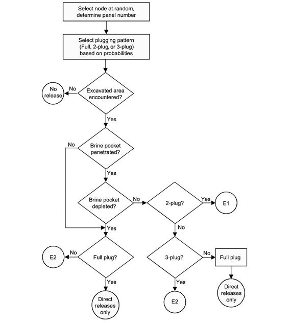
Figure PA- 33. Logic Diagram for Determining the Intrusion Type

The time and location of the previous intrusion is used to determine distance from the current intrusion and depends on the repository condition, which is determined by the intrusion of greatest consequence across all panels prior to the current intrusion. E1 intrusions are assumed to be of greater consequence than E2 intrusions. The previous intrusion is selected by finding the closest panel (same, adjacent, nonadjacent) whose intrusion condition, excluding the current intrusion, is equal to the repository condition. The time of the previous intrusion is the time of the most recent intrusion with the greatest consequence and closest distance. Likewise, the condition of each panel is equal to the intrusion of greatest consequence into the panel prior to the current intrusion.

PA-6.8.5 CCDF Construction

For each vector v _su,k in the space of subjective uncertainty, the code CCDFGF samples a sequence x _st,i , i = 1, 2, ¼, nR of futures. In PA, nR = 10,000; this number of futures is sufficient to adequately estimate the mean CCDF of total releases for comparison with the boundary line specified in section 191.13, as demonstrated in Section PA-9.0. A release f(x _st,i ) for each future is then constructed as described in Section PA-6.8.1, Section PA-6.8.2, and Section PA-6.8.3. Once the f(x _st,i ) are evaluated, the CCDF can be approximated as indicated in Equation (PA.321).

(PA.321)

A binning technique is used to construct the desired CCDF: the consequence axis is divided into a sequence of bins, and the number of values for f(x _st,i ) falling in each bin is accumulated. In addition, all values for f(x _st,i ) are saved and subsequently ordered to provide an alternative method for constructing the CCDFs. In addition to the total CCDF for all releases, it will be possible to obtain CCDFs for individual release modes (e.g., cuttings, spallings, DBRs, to Culebra, through MBs, through Culebra). The logic diagram for CCDF production is shown in Figure PA-34.

The CCDF construction indicated in this section is for a single sample element v _su,k of the form indicated in conjunction with Equation (PA.305). Repeated generation of CCDFs for individual sample elements v _su,k , i.e. for the vectors representing epistemic uncertainty in the model results, will lead to the distribution of complete CCDFs.

PA-6.9 Sensitivity Analysis

Evaluating one or more of the models discussed in Section PA-4.0 with the LHS in Equation (PA.305) creates a mapping

, k = 1, 2, ¼, nLHS (PA.322)

from analysis inputs (i.e., v _su,k ) to analysis results (i.e., y(v _su,k )), where y _su,k denotes the results obtained with the model or models under consideration. In other words, for each vector of parameters samples, there is a corresponding CCDF of releases, y(v _su,k ). A vector notation is used for y because, in general, a large number of predicted results are produced by each of the models used in PA. Sensitivity analysis explores the mapping in Equation (PA.322) to determine how the uncertainty in individual elements of v _su,k affects the uncertainty in individual elements of y(v _su,k ). Understanding how uncertainty in analysis inputs affects analysis results aids in understanding PA and improving the models for future PAs. In some cases, sensitivity analysis results are based on pooling the results obtained for the three replicated LHSs (i.e., R1, R2, R3) discussed in Section PA-6.4. In other cases, the sensitivity analysis is based on the results for each replicate, and statistics are compared across the three replicates. Note that pooling LHS replicates that include correlated variables can introduce a small bias into the statistics, although there are methods that allow for correlated variables when pooling replicates (Sallaberry, Helton, and Hora 2006).

Three principal techniques are used in the sensitivity analysis: scatterplots, regression analyses to determine standardized regression coefficients and partial correlation coefficients, and stepwise regression analyses. Each technique is briefly discussed.

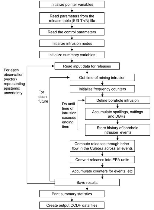
Figure PA- 34. Processing of Input Data to Produce CCDFs

PA-6.9.1Scatterplots

Scatterplots, the simplest sensitivity analysis technique, are performed by plotting the points

, k = 1, 2, ¼, nLHS (PA.323)

for each element v _j of _su . The resulting plots can reveal relationships between y and the elements of _su . Scatterplots can be effective at revealing nonlinear relationships or threshold values. Examining such plots when LHS is used can be particularly revealing because of the full stratification over the range of each input variable. Iman and Helton (Iman and Helton 1988) provide an example where the scatterplots revealed a rather complex pattern of variable interactions.

PA-6.9.2 Regression Analysis

A more formal investigation of the mapping in Equation (PA.322) can be based on regression analysis. In this approach, a model of the form

(PA.324)

is developed from the mapping between analysis inputs and analysis results shown in Equation (PA.322), where the x _j are the input variables under consideration and the b _j are coefficients that must be determined. The coefficients b _j and other aspects of the regression model's construction in Equation (PA.324) can indicate the importance of the individual variables x _j with respect to the uncertainty in y. The PA employs the method of least squares to determine the coefficients b _j (Myers 1986).

Often the regression in Equation (PA.324) is performed after the input and output variables are normalized to mean zero and standard deviation one. The resulting coefficients b _j are called standardized regression coefficients (SRCs). When the x _j are independent, the absolute value of the SRCs can provide a measure of variable importance. Specifically, the coefficients provide a measure of importance based on the effect of moving each variable away from its expected value by a fixed fraction of its standard deviation while retaining all other variables at their expected values.

Partial correlation coefficients (PCCs) can also measure the linear relationships between the output variable y and the individual input variables. The PCC between y and an individual variable x _p is obtained through a sequence of regression models. First, the following two regression models are constructed:

(PA.325)

The results of the two preceding regressions are then used to define the new variables and . By definition, the PCC between y and x _p is the correlation coefficient between and . Thus, the PCC provides a measure of the linear relationship between y and x _p with the linear effects of the other variables removed.

Regression and correlation analyses often perform poorly when the relationships between the input and output variables are nonlinear. This is not surprising, as such analyses assume linear relationships between variables. The problems associated with poor linear fits to nonlinear data can be avoided by use of the rank transformation (Iman and Conover 1979). The rank transformation is a simple concept: data are replaced with their corresponding ranks, and then the usual regression and correlation procedures are performed on these ranks. Specifically, the smallest value of each variable is assigned Rank 1, the next largest value is assigned Rank 2, and so on up to the largest value, which is assigned the rank m, where m denotes the number of observations. The analysis is then performed with these ranks used as the values for the input and output variables. A formal development of PCCs and the relationships between PCCs and SRCs is provided by Iman, Shortencarier, and Johnson (Iman, Shortencarier, and Johnson 1985).

PA-6.9.3 Stepwise Regression Analysis

Stepwise regression analysis provides an alternative to constructing a regression model containing all the input variables. With this approach, a sequence of regression models is constructed. The first regression model contains the single input variable with the largest impact on the uncertainty in the output variable (i.e., the input variable that has the largest correlation with the output variable y). The second regression model contains the two input variables with the largest impact on the output variable: the input variable from the first step, plus whichever of the remaining variables has the largest impact on uncertainty not accounted for by the first variable (i.e., the input variable that has the largest correlation with the uncertainty in y that cannot be accounted for by the first variable). Additional models in the sequence are defined in the same manner, until further models are unable to meaningfully increase the amount of uncertainty that can be accounted for in the output variable.

Stepwise regression analysis can provide insights into the importance of the individual variables. First, the order in which the variables are selected in the stepwise procedure indicates their importance, with the most important variable being selected first, the next most important variable being selected second, and so on. Second, the R² values at successive steps of the analysis also measure variable importance by indicating how much of the uncertainty in the dependent variable can be accounted for by all variables selected at each step. When the input variables are uncorrelated, the differences in the R² values for the regression models constructed at successive steps equals the fraction of the total uncertainty in the output variable accounted for by the individual input variable added at each step. Third, the absolute values of the SRCs in the individual regression models indicate variable importance. Further, the sign of an SRC indicates whether the input and output variable tend to increase and decrease together (a positive coefficient) or tend to move in opposite directions (a negative coefficient).

PA-7.0 Results for the Undisturbed Repository

The PA tabulates releases from the repository for undisturbed conditions. Releases from the undisturbed repository to the accessible environment fall under two sets of protection requirements. The first, as set forth in section 191.15, protects individuals from radiological exposure; the second, in 40 CFR Part 191 Subpart C, protects groundwater resources from contamination. This section shows how the WIPP complies with these two requirements by presenting brine and gas flow (BRAGFLO) and radionuclide transport (NUTS) results from modeling the undisturbed repository. For the undisturbed repository, radionuclide transport through the repository shafts to the Culebra, and lateral radionuclide transport through the marker beds and across the LWB, are the only potential release mechanisms. The results discussed in Section PA-7.2 show that there are no releases to the accessible environment from the undisturbed repository. Results of the CRA-2014 PA for the undisturbed repository are summarized in Camphouse et al. (Camphouse et al. 2013). The overall structure of the CRA-2014 PA is summarized in Section PA-1.1.

PA-7.1 Salado Flow

This section summarizes the Salado flow calculation results for the undisturbed (S1-BF) scenario (see Table PA-20 for an explanation of the BRAGFLO scenarios). The Salado flow model represents the repository as five regions in the numerical grid: three waste-filled regions (the Waste Panel, South RoR, and North RoR in Figure PA-12) and two excavated regions with no waste (the operations area and experimental area in Figure PA-12). A detailed presentation of the CRA-2014 PA Salado flow results can be found in Camphouse (Camphouse 2013c).

In undisturbed conditions, pressure strongly influences the extent to which contaminated brine might migrate from the repository to the accessible environment. Pressures and brine saturations in repository waste regions are important quantities relevant to direct release mechanisms considered in the WIPP PA. Spallings releases depend directly on repository pressure. Direct brine releases (DBRs) depend on both repository pressure and brine saturation. Waste region pressures and brine saturations obtained for undisturbed conditions are used to generate initial conditions for the spallings and DBR models (Section PA-8.5.2 and Section PA-8.5.3, respectively). Consequently, results for these quantities in the undisturbed repository can impact results seen for the disturbed scenarios investigated in the WIPP PA.

Figure PA-35 through Figure PA-40 show the waste region pressures for scenario S1-BF of the CRA-2014 PA. Overall mean pressure curves shown for the CRA-2009 PABC and the CRA-2014 PA are obtained by forming the average of all 300 vector realizations. Over time, repository pressures increase due to several factors: rapid initial creep closure of rooms, initial inflow of brine causing gas generation due to corrosion, and availability of CPR material to produce gas by microbial degradation. Changes included in the CRA-2014 PA yield a reduction in the mean pressure calculated for undisturbed repository waste areas as compared to the CRA-2009 PABC. The expanded mined volume in the repository experimental area contributes somewhat to this reduction, but it is primarily due to reduced gas generation seen in the CRA-2014 PA results. The revised iron corrosion rate utilized in the CRA-2014 PA results in slower gas production due to iron corrosion (on average). The addition of MgO chemistry in the revised water balance implementation also reduces the amount of free water available for gas production by iron corrosion and microbial degradation of cellulose. The sequestration of free water further reduces gas production, and consequently pressure, in repository waste areas (Camphouse 2013c).

Figure PA- 35. Horsetail Plot of Waste Panel Pressure, Scenario S1-BF, CRA-2014 PA

Figure PA- 36. Overall Means of Waste Panel Pressure, Scenario S1-BF

Figure PA- 37. Horsetail Plot of SRoR Pressure, Scenario S1-BF, CRA-2014 PA

Figure PA- 38. Overall Means of SRoR Pressure, Scenario S1-BF

Figure PA- 39. Horsetail Plot of NRoR Pressure, Scenario S1-BF, CRA-2014 PA

Figure PA- 40. Overall Means of NRoR Pressure, Scenario S1-BF

The trend toward waste region pressure reduction in the CRA-2014 PA yields a corresponding increase (on average) in cumulative brine inflow to repository waste regions (cumulative brine inflow includes inflow from the surrounding rock and adjacent panels). Increases in waste region brine inflow are more pronounced for waste panels at lower elevation due to the 1° dip in elevation north-to-south that is implemented in the Salado flow model. The changes in brine inflow to repository waste regions have a direct impact on the brine saturations calculated for those areas. Waste region brine saturations obtained in the CRA-2014 PA are shown in Figure PA-41 to Figure PA-46. Overall mean brine saturation curves shown for the CRA-2009 PABC and the CRA-2014 PA are obtained by forming the average of all 300 vector realizations. As seen in Figure PA-41 to Figure PA-46, brine saturations tend to be higher in the waste panel at lowest elevation, with brine saturations typically being lower in the SRoR and NRoR than those seen in the separately modeled waste panel. Moreover, waste areas at higher elevation, such as the SRoR and the NRoR, have lower mean brine saturations in the CRA-2014 PA results as compared to the CRA-2009 PABC, especially in the first 2000 years. This is due to water sequestration in the refined water balance implementation and the combination of the 1-degree repository downdip and more permeable panel closures at early times. Waste panels at lowest elevation, such as the separately modeled waste panel in BRAGFLO, have a lower mean brine saturation at early times as compared to the CRA-2009 PABC. However, the mean waste panel brine saturation gradually increases until it becomes greater than that seen in the CRA-2009 PABC at roughly 750 years. As the SRoR and NRoR together represent nine of the ten repository waste panels, the sequestration of brine in the refined water budget implementation yields a repository that tends to be drier overall for undisturbed conditions as compared to the CRA-2009 PABC (Camphouse 2013c).

Figure PA- 41. Horsetail Plot of Waste Panel Brine Saturation, Scenario S1-BF, CRA-2014 PA

Figure PA- 42. Overall Means of Waste Panel Brine Saturation, Scenario S1-BF

Figure PA- 43. Horsetail Plot of SRoR Brine Saturation, Scenario S1-BF, CRA-2014 PA

Figure PA- 44. Overall Means of SRoR Brine Saturation, Scenario S1-BF

Figure PA- 45. Horsetail Plot of NRoR Brine Saturation, Scenario S1-BF, CRA-2014 PA

Figure PA- 46. Overall Means of NRoR Brine Saturation, Scenario S1-BF

The repository shaft is modeled in the WIPP PA as being directly between the operations and experimental regions of the repository. Consequently, the pressure in these repository regions impacts the volume of brine moved up the shaft toward the ground surface, shown in Figure PA-47 and Figure PA-48. The trend toward lower pressure in repository waste regions in the CRA-2014 PA translates to a similar trend toward pressure reduction in the repository operations and experimental regions. The trend toward lower pressure in these areas results in an overall reduction to the mean cumulative brine flow up the shaft in the CRA-2014 PA.

In the CRA-2009 PABC, vector 53 of replicate 1 had the highest total cumulative brine flow to the LWB for the undisturbed repository. It was the only vector that was screened in as a source of radionuclide transport through the Salado marker beds and across the LWB in the NUTS calculation. Vector 53 of replicate 1 also has the highest cumulative brine flow to the LWB for the undisturbed repository in the CRA-2014 PA. However, the maximum brine outflow across the LWB associated with this vector is reduced in the CRA-2014 PA due to reduced pressures seen for the undisturbed repository in the CRA-2014 PA. In addition, brine flow across the LWB for this vector starts at roughly 6,500 years post-closure in the CRA-2014 PA as compared to roughly 3,000 years post-closure in the CRA-2009 PABC (Figure PA-49).

Figure PA- 47. Horsetail Plot of Brine Flow up the Shaft, Scenario S1-BF, CRA-2014 PA

Figure PA- 48. Overall Means of Brine Flow up the Shaft, Scenario S1-BF

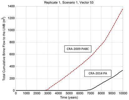
Figure PA- 49. Comparision of Brine Flow Across the LWB, Scenario S1-BF, CRA-2009 PABC and CRA-2014 PA

PA-7.2 Radionuclide Transport

This section summarizes the radionuclide transport results for the undisturbed repository, both up the shaft to the Culebra and through the Salado to the LWB. Radionuclide transport in the undisturbed scenario is calculated by the code NUTS. Kim (Kim 2013a) presents a detailed analysis of the NUTS results for the CRA-2014 PA.

Screening runs using a conservative tracer determine which vectors have the potential to transport radionuclides to the accessible environment. Full Salado transport simulations are then performed for all screened-in vectors that have the potential to transport radionuclides to the accessible environment. In the CRA-2009 PABC, only vector 53 of replicate 1 was screened in for the radionuclide transport calculation in the undisturbed scenario. In the CRA-2014 PA, no vectors exceeded the NUTS screening step for the undisturbed repository (Kim and Camphouse 2013). As discussed in the preceding section, vector 53 of replicate 1 also has the highest cumulative brine flow to the LWB for the undisturbed repository in the CRA-2009 PA and the CRA-2014 PA. However, the maximum brine outflow across the LWB associated with this vector is reduced in the CRA-2014 PA due to reduced pressures seen for the undisturbed repository. Brine outflows across the LWB associated with this vector also begin at later times in the CRA-2014 PA. Consequently, no vectors exceeded the NUTS screening criterion, resulting in no radionuclide transport through the Salado to the LWB in the CRA-2014 PA. Similarly, no vectors showed radionuclide transport through the shafts to the Culebra (Kim 2013a).

As no radionuclide transport to the accessible environment occurred in the CRA-2014 PA, there are no releases associated with the undisturbed scenario in the CRA-2014 PA.

PA-8.0 Results for a Disturbed Repository

The WIPP repository might be disturbed by exploratory drilling for natural resources during the 10,000-year regulatory period. Drilling could create additional pathways for radionuclide transport, especially in the Culebra, and could release material directly to the surface. In addition, mining for potash within the LWB might alter flow in the overlying geologic units and locally accelerate transport through the Culebra. The disturbed scenarios used in PA modeling capture the range of possible releases resulting from drilling and mining.

Total releases are computed by the code CCDFGF. Total releases comprise transport releases and direct releases. Transport releases generally involve movement of radionuclides up an abandoned borehole into the Culebra, then through the Culebra to the LWB. Transport of radionuclides to the Culebra is computed using the codes NUTS and PANEL (see Section PA-6.7.2 and Section PA-6.7.3) using the brine flows computed by BRAGFLO (see Section PA-6.7.1). Radionuclide transport through the Culebra is computed by the code SECOTP2D (see Section PA-6.7.8) using flow fields calculated by MODFLOW (see Section PA-6.7.7).

Direct releases occur at the time of a drilling intrusion and include releases of solids (cuttings, cavings, and spallings) computed using the code CUTTINGS_S (see Section PA-6.7.4) and DBRs computed using BRAGFLO (see Section PA-6.7.6). Pressure and brine saturation within the waste areas are used as initial conditions for the direct release models. Results from the undisturbed repository (see Section PA-7.0) are used as the initial conditions for the first intrusion. To calculate initial conditions for subsequent intrusions, and to compute the source of radionuclides for transport in the Culebra, BRAGFLO uses a set of drilling scenarios to calculate conditions within the repository after an intrusion (see Section PA-6.7.6).

This section first summarizes the scenarios used to represent drilling intrusions and the resulting repository conditions calculated by BRAGFLO. Transport releases are presented next, followed by cuttings, cavings, spallings, and DBRs. The CRA-2014 PA results obtained for the disturbed repository are summarized in Camphouse et al. (Camphouse et al.2013).

PA-8.1 Drilling Scenarios

As shown in Table PA-20, the PA considers two types of drilling intrusions: E1 and E2. The E1 intrusion scenario represents the possibility that a borehole creates a pathway between the repository and a pressurized brine reservoir located within the underlying Castile formation. The E2 intrusion scenario represents a borehole that intrudes into the repository, but does not connect the repository with an underlying brine reservoir. Repository conditions are calculated for the E1 intrusion scenario at 350 and 1,000 years, and are referred to as the BRAGFLO S2-BF and S3-BF scenarios, respectively. The BRAGFLO Scenarios S4-BF and S5-BF represent E2 intrusions that occur at 350 and 1,000 years, respectively. An additional BRAGFLO scenario, S6-BF, simulates the effects of an E2 intrusion at 1,000 years followed by an E1 intrusion 1,000 years later into the same panel.

PA-8.2 Mining Scenarios

Long-term releases within the Culebra could be influenced by future mining activities that remove all the known potash reserves within the LWB and cause the transmissivity within the overlying Culebra to change (see Section PA-4.8). The full mining of known potash reserves within the LWB in the absence of AICs and PICs is modeled as a Poisson process, with a rate of 10^- ⁴ yr^- ¹ (see Section PA-3.9). For any particular future, this rate is used to determine a time at which full mining has occurred. Flow fields are calculated for the Culebra for two conditions: partial mining, which assumes all potash has been mined from reserves outside the LWB; and full mining, which assumes all reserves have been mined both inside and outside the LWB. Radionuclide transport through the Culebra uses the partial-mining flow fields prior to the time at which full mining has occurred and the full-mining flow fields after that time.

PA-8.3 Salado Flow

This section summarizes the results of the Salado flow calculations for the disturbed scenarios. Camphouse (Camphouse 2013c) provides a detailed presentation of BRAGFLO results obtained in the CRA-2014 PA.

PA-8.3.1 Salado Flow Results for E1 Intrusion Scenarios

Results are now presented for disturbed scenario S2-BF. Results presented for this scenario are representative of those calculated for E1 intrusion scenarios (scenarios S2-BF and scenario S3-BF), with the only difference being the time of intrusion. In the results that follow, trends discussed for scenario S2-BF also apply to scenario S3-BF. Results presented in this section are limited to those calculated for the intruded waste panel. Quantities calculated for the SRoR and NRoR in scenario S2-BF are similar to those calculated and previously discussed for undisturbed conditions because the panel closures in the CRA-2014 PA are tighter than the Option D closures in the CRA-2009 PABC.

Scenario S2-BF represents an E1 intrusion at 350 years. The horsetail plot of waste panel pressure obtained for the 300 vector realizations of the CRA-2014 PA is shown in Figure PA-50. The overall mean waste panel pressure curves obtained in the CRA-2014 PA and the CRA-2009 PABC are plotted together in Figure PA-51. The reduction in pressure (on average) for the undisturbed repository translates to lower porosity (on average) in repository waste regions at the time of intrusion (Camphouse 2013c). The trend toward reduced porosity at the time of intrusion results in increased pressure in the waste panel after it is connected to highly pressurized Castile brine during the intrusion, because of the reduced volume for the brine to flow into. The replacement of the Option D PCS with the ROMPCS that has "tighter" long-term properties also contributes to this pressure increase. The mean waste panel pressure obtained in the CRA-2014 PA remains higher than that seen in the CRA-2009 PABC for a period of time after the intrusion, but eventually falls below the CRA-2009 PABC result at roughly 6200 years (Figure PA-51). The impact of the revised iron corrosion rate implemented in the CRA-2014 PA results in a reduction (on average) to the rate of gas production due to iron corrosion. Gas generation due to iron corrosion is the dominant gas production mechanism in both the CRA-2014 PA and the CRA-2009 PABC. The reduction (on average) in the rate of gas production due to iron corrosion in the CRA-2014 PA yields a corresponding decrease in the rate of mean gas generation in the waste panel, resulting in the eventual reduction in waste region pressure as compared to the CRA-2009 PABC.

The reduction in mean waste panel pressure in the CRA-2014 PA for the undisturbed repository allows for increased brine inflow to the waste panel up to the time of intrusion. The increased brine inflow to the waste panel has a direct impact on waste panel brine saturation. The horsetail plot of waste panel brine saturation obtained in the CRA-2014 PA is shown in Figure PA-52. The overall mean waste panel brine saturation curves obtained in the CRA-2014 PA and the CRA-2009 PABC are plotted together in Figure PA-53. The increased mean waste panel brine inflow seen in the CRA-2014 PA as compared to the CRA-2009 PABC results in a corresponding increase in the CRA-2014 PA mean waste panel brine saturation following the E1 intrusion at 350 years.

Brine flow up the intrusion borehole potentially results in contaminated brine being transported to the ground surface following the intrusion as well as lateral transport of contaminated brine through the Culebra and across the LWB. The horsetail plot of cumulative brine flow up the intrusion borehole obtained in the CRA-2014 PA is shown in Figure PA-54. Overall means for this quantity obtained in the CRA-2014 PA and the CRA-2009 PABC are plotted together in Figure PA-55. The increased waste panel brine saturation in the CRA-2014 PA results, combined with the increase in mean waste panel pressure for a period of time after the intrusion, yields an increase in the overall mean obtained for brine flow up the intrusion borehole in the CRA-2014 PA as compared to the CRA-2009 PABC.

Figure PA- 50. Horsetail Plot of Waste Panel Pressure in the CRA-2014 PA, Scenario S2-BF

Figure PA- 51. Overall Means of Waste Panel Pressure, Scenario S2-BF

Figure PA- 52. Horsetail Plot of Waste Panel Brine Saturation in the CRA-2014 PA, Scenario S2-BF

Figure PA- 53. Overall Means of Waste Panel Brine Saturation, Scenario S2-BF

Figure PA- 54. Horsetail Plot of Cumulative Brine Flow up the Intrusion Borehole in the CRA-2014 PA, Scenario S2-BF

Figure PA- 55. Overall Means of Brine Flow up the Borehole, Scenario S2-BF

PA-8.3.2 Salado Flow Results for E2 Intrusion Scenarios

Results are now presented for disturbed scenario S4-BF. Scenario S4-BF represents an E2 intrusion at 350 years. Results presented for this scenario are representative of those calculated for E2 intrusion scenarios (scenarios S4-BF and scenario S5-BF), with the only difference being the time of intrusion. In the results that follow, trends discussed for scenario S4-BF also apply to scenario S5-BF. Results presented in this section are limited to those calculated for the intruded waste panel. Quantities calculated for the SRoR and NRoR are similar to those calculated and previously discussed for undisturbed conditions because of the tighter panel closures.

The horsetail plot of waste panel pressure obtained for the 300 vector realizations of scenario S4-BF in the CRA-2014 PA is shown in Figure PA-56. The overall means of waste panel pressure obtained in the CRA-2014 PA and the CRA-2009 PABC are plotted together in Figure PA-57. The refined iron corrosion rate and water budget implementation utilized in the CRA-2014 PA result in a reduction in the overall mean waste panel pressure as compared to the CRA-2009 PABC for undisturbed conditions. Consequently, at the time of the E2 intrusion, the mean waste panel pressure is lower in the CRA-2014 PA result than in the CRA-2009 PABC, and is also lower 200 years later when the borehole plugs fail. The result is a lower scenario S4-BF mean pressure in the CRA-2014 PA than in the CRA-2009 PABC. The trend toward reduced pressure in the CRA-2014 PA scenario S4-BF results in a corresponding trend toward increased brine flow to the waste panel prior to the E2 intrusion at 350 years, as well as increased brine inflow to the panel after the borehole plugs fail at 550 years. As seen in the results for the undisturbed repository, brine sequestration due to MgO hydration yields a reduced mean brine saturation in the waste panel prior to the intrusion at 350 years, even though the brine inflow at early times is higher in the CRA-2014 PA result. The increased inflow of brine following the intrusion yields an increased mean brine saturation in the CRA-2014 PA results as more brine becomes available in the waste panel than can be sequestered by MgO hydration. The horsetail plot of waste panel brine saturation obtained in scenario S4-BF in the CRA-2014 PA is shown in Figure PA-58. The overall means of waste panel brine saturation obtained in the CRA-2014 PA and the CRA-2009 PABC are plotted together in Figure PA-59. The mean cumulative brine flow up the intrusion borehole is similar, but slightly higher, in the CRA-2014 PA as compared to the CRA-2009 PABC. The horsetail plot of cumulative brine flow up the intrusion borehole obtained in scenario S4-BF of the CRA-2014 PA is shown in Figure PA-60. Overall means for this quantity obtained in the CRA-2014 PA and the CRA-2009 PABC are plotted together in Figure PA-61.

Figure PA- 56. Horsetail Plot of Waste Panel Pressure in the CRA-2014 PA, Scenario S4-BF

Figure PA- 57. Overall Means of Waste Panel Pressure, Scenario S4-BF

Figure PA- 58. Horsetail Plot of Waste Panel Brine Saturation in the CRA-2014 PA, Scenario S4-BF

Figure PA- 59. Overall Means of Waste Panel Brine Saturation, Scenario S4-BF

Figure PA- 60. Horsetail Plot of Cumulative Brine Flow up the Intrusion Borehole in the CRA-2014 PA, Scenario S4-BF

Figure PA- 61. Overall Means of Brine Flow up the Borehole, Scenario S4-BF

PA-8.3.3 Salado Flow Results for the Multiple Intrusion Scenario

BRAGFLO scenario S6-BF models an E2 intrusion occurring at 1000 years, followed by an E1 intrusion into the same panel at 2000 years. Calculated brine flows up the intrusion borehole obtained in scenario S6-BF are used in PA code PANEL to determine the radionuclide source term to the Culebra for the multi-intrusion case. The overall mean of cumulative brine flow up the intrusion borehole in scenario S6-BF (Figure PA-63) is increased in the CRA-2014 PA as compared to the CRA-2009 PABC, with the increase similar to that seen for the E1 intrusion results (Figure PA-55). The horsetail plot of cumulative brine flow up the intrusion borehole obtained in the CRA-2014 PA for scenario S6-BF is shown in Figure PA-62.

Figure PA- 62. Horsetail Plot of Cumulative Brine Flow up the Intrusion Borehole in the CRA-2014 PA, Scenario S6-BF

Figure PA- 63. Overall Means of Brine Flow up the Borehole, Scenario S6-BF

PA-8.4 Radionuclide Transport

In the disturbed scenarios, radionuclide transport in the Salado is calculated by the code NUTS (see Section PA-6.7.2). Radionuclide transport from the Salado to the Culebra is calculated by NUTS and PANEL (see Section PA-6.7.2 and Section PA-6.7.3). Radionuclide transport within the Culebra is calculated by SECOTP2D (see Section PA-6.7.8). For all radionuclide transport calculations, mobilized concentrations of radionuclides in Salado and Castile brines are computed by the code PANEL (see Section PA-6.7.3).

This section summarizes the radionuclide transport results for the disturbed scenarios. Camphouse (Camphouse 2013c) describes the brine and gas flow in the Salado. Detailed analysis of the radionuclide transport in the Salado is presented in Kim (2013a). Kim (2013b) provides an analysis of the mobilized concentrations of radionuclides in Salado and Castile brines. Appendix TFIELD-2014 and Kuhlman (2010) present an analysis of the flow and radionuclide transport within the Culebra.

PA-8.4.1 Radionuclide Mobilized Concentrations

The code PANEL calculates the time-varying concentration of radionuclides mobilized in brine, either as dissolved isotopes or as isotopes sorbed to mobile colloids (see Equation (PA.124) and Equation (PA.125)). Two different brines are considered: GWB, a magnesium-rich interstitial brine present in the Salado Formation; and ERDA-6, a sodium-rich brine in the Castile. Radionuclide solubility in the two brines can be considerably different. Before an E1 intrusion, PA assumes that the brine in the repository is GWB; after an E1 intrusion, brine in the repository is assumed to be ERDA-6. Baseline radionuclide solubilities are calculated using multiples of the minimum brine volume (17,400 m³) necessary for a DBR to occur (Brush and Domski 2013b). Brine volumes of 1x, 2x, 3x, 4x, and 5x this minimum necessary brine volume are used in the calculation of baseline radionuclide solubilities in ERDA-6 brine and GWB, and these solubilities are listed in Kicker and Herrick (Kicker and Herrick 2013), Table 27.

Figure PA-64 and Figure PA-65 show the concentration of radioactivity mobilized in Salado brine as a function of time for all vectors in replicate 1 of the CRA-2014 PA. Figure PA-64 shows results obtained using baseline solubilities corresponding to the minimum brine volume of 17,400 m³ (denoted as BV1 in that figure). Figure PA-65 shows results obtained using baseline solubilities corresponding to 5x the minimum brine volume (denoted as BV5 in that figure). Analogous results for Castile brine are shown in Figure PA-66 and Figure PA-67. As seen in those figures, radionuclide concentrations are reduced by roughly a factor of four from the minimum brine volume (BV1) to five times the minimum brine volume (BV5). Concentrations are expressed as EPA units/m³ to combine the radioactivity of different isotopes. At early times (before 2000 years), the total mobilized concentrations (in both Salado and Castile brines) have their highest values because of the contribution of americium. After about 4000 years, the contribution from americium is much reduced because of the decay of ²⁴¹Am. After about 4000 years, the total mobilized concentrations are dominated by plutonium, with concentrations of uranium and thorium being orders of magnitude lower (Kim 2013b).

The CRA-2014 PA results for total mobilized concentrations show a similar variability to what was obtained in the CRA-2009 PABC. However, total mobilized concentrations obtained in the CRA-2014 PA decrease as the brine volume increases. This trend is expected to reduce releases associated with large DBR volumes in the CRA-2014 PA as compared to the CRA-2009 PABC.

Figure PA- 64. CRA-2014 PA Total Mobilized Concentrations in Salado Brine, Replicate 1, BV1

Figure PA- 65. CRA-2014 PA Total Mobilized Concentrations in Salado Brine, Replicate 1, BV5

Figure PA- 66. CRA-2014 PA Total Mobilized Concentrations in Castile Brine, Replicate 1, BV1

Figure PA- 67. CRA-2014 PA Total Mobilized Concentrations in Castile Brine, Replicate 1, BV5

PA-8.4.2 Transport through MBs and Shaft

In the disturbed scenarios, none of the 300 realizations obtained in the CRA-2014 PA resulted in releases through the the markerbeds that exceed the screening limit of 1 × 10^-7 kg/m³. In the CRA-2009 PABC, vector 53 of replicate 1 exceeded this limit for scenario S2-BF. As was the case in the CRA-2009 PABC, no realization showed transport of radionuclides through the shaft to the Culebra in the CRA-2014 PA.

PA-8.4.3 Transport to the Culebra

Radionuclide transport to the Culebra via a single intrusion borehole (disturbed scenarios S2-BF, S3-BF, S4-BF, and S5-BF) is modeled with the code NUTS (Section PA-4.3). Transport to the Culebra in the multiple intrusion scenario (S6-BF) is modeled with the code PANEL (Section PA-4.4). Detailed discussion of the radionuclide transport to the Culebra calculations can be found in Kim (Kim 2013a).

Figure PA-68 through Figure PA-72 show cumulative radioactivity transported up the borehole to the Culebra for the intrusion scenarios modeled with BRAGFLO. Transport to the Culebra is larger and occurs for more vectors in the S2-BF, S3-BF and S6-BF scenarios (with E1 intrusions) than in the S4-BF or S5-BF scenarios (E2 intrusions only). Most transport to the Culebra occurs over a relatively short period of time immediately after the borehole intrusion. For some E2 cases the releases are delayed because of the need to build up sufficient gas pressure. For the multiple intrusion scenario (S6-BF), only 5 vectors show radionuclide transport resulting from the E2 intrusion at 1,000 years; most radionuclide transport occurs immediately after the E1 intrusion at 2,000 years.

Radionuclide transport releases to the Culebra obtained in the CRA-2014 PA exhibit larger maximum and average values than were obtained in the CRA-2009 PABC (Kim 2013a). As seen in the Salado flow results already discussed, brine flows up the intrusion borehole are larger (on average) in the CRA-2014 PA than in the CRA-2009 PABC. Only the baseline radionuclide solubilities corresponding to the minimum brine volume necessary for a DBR are used in the CRA-2014 PA Salado transport calculation to keep the computational expense associated with NUTS calculations at a feasible level. Baseline solubilities corresponding to this volume of brine in the CRA-2009 PABC and the CRA-2014 PA are similar. However, the mean and maximum values of the solubility uncertainty distribution for +IV actinides increased in the CRA-2014 PA. This, combined with the overall trend toward increased brine flow up the intrusion borehole, results in a trend toward increased radionuclide transport releases to the Culebra for CRA-2014 PA disturbed scenarios.

Figure PA- 68. CRA-2014 PA Cumulative Transport Release to the Culebra, Scenario S2-BF

Figure PA- 69. CRA-2014 PA Cumulative Transport Release to the Culebra, Scenario S3-BF

Figure PA- 70. CRA-2014 PA Cumulative Transport Release to the Culebra, Scenario S4-BF

Figure PA- 71. CRA-2014 PA Cumulative Transport Release to the Culebra, Scenario S5-BF

Figure PA- 72. CRA-2014 PA Cumulative Transport Release to the Culebra, Scenario S6-BF

PA-8.4.4 Transport through the Culebra

As none of the changes included in the CRA-2014 PA impact Culebra transport, the CRA-2014 PA uses Culebra transport results obtained in the CRA-2009 PABC. The CRA-2009 PABC Culebra transport calculation included a number of changes as compared to Culebra transport results used in the CRA-2009 PA. These changes included:

Changes in the definition of minable potash
Reductions to the lower limits of the matrix distribution coefficients (K _d ) for Am(III), Pu(III), Pu(IV), Th(IV), and U(IV)
Updates to the Culebra transmissivity fields

Radionuclide transport th _r ough the Culebra for a given set of uncertain parameters is calculated with the code SECOTP2D (see Section PA-6.7.8). Note that the total release of radionuclides across the LWB at the Culebra for given futures is calculated with the code CCDFGF by convolving the SECOTP2D results with the radionuclide transport to the Culebra calculated by NUTS and PANEL. This section discusses the SECOTP2D results; total releases through the Culebra are presented in Section PA-9.4.

Culebra radionuclide transport calculations were performed for three replicates of 100 vectors each for both partial-mining and full-mining scenarios (600 total simulations). Each of the 600 radionuclide transport simulations used a unique flow field computed separately with the code MODFLOW 2000 (see Kuhlman 2010). The partial-mining scenario assumes the extraction of all potash reserves outside the LWB, while the full-mining scenario assumes that all potash reserves both inside and outside the LWB are exploited.

In each radionuclide transport simulation, 1 kg of each of four radionuclides (²⁴¹Am, ²³⁴U, ²³⁰Th, and ²³⁹Pu) are released in the Culebra above the center of the waste panel area. Radionuclide transport of the ²³⁰Th daughter product of ²³⁴U decay is calculated and tracked as a separate species. In the following discussion, ²³⁰Th will refer to the ²³⁴U daughter product and ²³⁰ThA will refer to that released at the waste panel area.

For the three replicates included in the CRA-2014 PA, the number of vectors with cumulative releases greater than 10^-9 kg criterion, established in the CCA, is shown in Table PA-25 for each radionuclide, under partial and full mining conditions. All SECOTP2D results, regardless of magnitude, are included in the calculation of releases from the Culebra. Under partial and full mining conditions, ²³⁴U has the highest number of vectors that surpassed the 10^-9 kg criterion, while ²⁴¹Am has the least number of vectors. A considerable increase is observed in the full mining scenario compared with the partial mining scenario, due to the increased proximity of the potash reserves within the LWB to the repository, which are extracted in the full mining scenario (Kuhlman 2010).

Table PA- 25. Number of Realizations with Radionuclide Transport to the LWB

# of vectors	Partial Mining			Full Mining
# of vectors	R1	R2	R3	R1	R2	R3
²⁴¹Am	0	0	0	8	10	3
²³⁹Pu	3	1	1	20	27	22
²³⁴U	11	14	12	48	50	47
²³⁰Th	5	10	6	36	38	42
²³⁰ThA	2	3	0	21	31	29

PA-8.5 Direct Releases

Direct releases occur at the time of a drilling intrusion, and include cuttings and cavings, spallings, and DBRs. This section presents an analysis of the volume released by each mechanism.

Kicker (Kicker 2013) provides additional information about the cuttings, cavings, and spallings releases calculated for the CRA-2014 PA. Malama (2013) provides a detailed analysis of DBRs in the CRA-2014 PA.

PA-8.5.1 Cuttings and Cavings

Cuttings and cavings are the solid waste material removed from the repository and carried to the surface by the drilling fluid during borehole drilling. Cuttings are the materials removed directly by the drill bit, and cavings are the material eroded from the walls of the borehole by shear stresses from the circulating drill fluid. The volume of cuttings and cavings material removed from a single drilling intrusion into the repository is assumed to be in the shape of a cylinder. The code CUTTINGS_S calculates the area of the base of this cylinder, and cuttings and cavings results in this section are reported in terms of these areas. The volumes of cuttings and cavings removed can be calculated by multiplying these areas with the initial repository height 3.96 m (BLOWOUT:HREPO).

The drill bit diameter (parameter BOREHOLE:DIAMMOD ) is specified to be 0.31115 meters in both the CRA-2009 PABC and the CRA-2014 PA. A cuttings area of 0.0760 m² is obtained for all vectors in both the CRA-2009 PABC and the CRA-2014 PA as both analyses use the same constant drill bit diameter value. A refined distribution for parameter BOREHOLE:TAUFAIL is implemented in the CRA-2014 PA, and is listed in Kicker and Herrick (Kicker and Herrick 2013), Table 4. A loguniform distribution having a minimum of 0.05 Pa, a mean of 10.5 Pa, and a maximum of 77.0 Pa was used to represent uncertainty in parameter BOREHOLE:TAUFAIL in the CRA-2009 PABC. A uniform distribution having a minimum of 2.22 Pa, a mean of 39.61 Pa, and a maximum of 77.0 Pa is used for this parameter in the CRA-2014 PA. Parameter BOREHOLE:TAUFAIL is used to represent the effective shear strength for erosion of WIPP waste (see Section PA-4.5.2); changes to it potentially impact cavings release areas.

Cuttings and cavings area statistics calculated in the CRA-2014 PA are shown in Table PA-26. The refinement to parameter BOREHOLE:TAUFAIL used in the CRA-2014 PA results in a shift toward a lower mean cavings area as well as a decrease in the overall number of vectors with nonzero cavings area in the CRA-2014 PA as compared to the PABC-2009.

Table PA- 26. CRA-2014 PA Cavings Area Statistics

Replicate	Minimum (m²)	Maximum (m²)	Mean (m²)	Number of Vectors without Cavings
R1	0.0	0.090	0.01	50
R2	0.0	0.090	0.01	44
R3	0.0	0.075	0.01	50

The uncertainty in cavings area arises primarily from the uncertainty in the shear strength of the waste (Kicker 2013). Lower shear strengths tend to result in larger cavings releases, and hence larger cuttings and cavings releases.

PA-8.5.2 Spallings

Calculating the volume of solid waste material released to the surface due to spallings from a single drilling intrusion into the repository is a two-part procedure. The code DRSPALL calculates the spallings volumes from a single drilling intrusion at four values of repository pressure (10, 12, 14, and 14.8 MPa). Following this, spallings volumes from a single intrusion are calculated using the code CUTTINGS_S; this code linearly interpolates the spallings volumes calculated using DRSPALL, based on the pressure calculated by BRAGFLO. Results from both of these calculations are documented in this section.

PA-8.5.2.1 DRSPALL Results

None of the changes implemented in the CRA-2014 PA affect the DRSPALL calculations, so the DRSPALL results used in the CRA-2009 PA were also used in the CRA-2014 PA. These results were generated by running DRSPALL for each of 100 vectors in 3 replicates and for 4 values of repository pressure (10, 12, 14, and 14.8 MPa; see Section PA-4.6.4). No spallings occurred at 10 MPa for any vector.

The uncertainty in the spallings volumes arises from four uncertain variables in the DRSPALL calculations: waste permeability, waste porosity, waste tensile strength, and waste particle diameter after tensile failure (Table PA-11). Figure PA-73 indicates that the largest spallings volumes occur when waste permeability is less than 1.0 × 10^- ¹³ m², but larger permeability values result in a higher frequency of nonzero spallings volumes. This observation can be explained as follows: the higher permeability values sampled result in smaller tensile stresses and less tensile failure, but promote fluidization. Lower permeability leads to greater tensile stresses and tensile failure, but failed material may not be able to fluidize at this low permeability.

Figure PA- 73. Scatterplot of Waste Permeability Versus Spallings Volume, CRA-2014 PA

Smaller particle diameter values (see Figure PA-74) tend to result in larger spallings volumes and a higher frequency of nonzero spallings volumes. The uncertainty in the spallings volumes from a single intrusion is largely determined by the uncertainty in these two parameters. Obvious correlations between spallings volumes and the other two parameters could not be established.

Figure PA- 74. Scatterplot of Waste Particle Diameter Versus Spallings Volume,
CRA-2014 PA

PA-8.5.2.2 CUTTINGS_S Results

Two factors directly affect the CUTTINGS_S calculation of spallings volumes for the drilling scenarios: the volumes calculated by DRSPALL and the repository pressures calculated by BRAGFLO.

Table PA-27 summarizes the statistics for the CRA-2014 PA spallings volumes. Results presented in that table are assessed over all three replicates, times, vectors, and drilling locations. The maximum spallings volumes obtained for scenarios S1-DBR, S4-DBR, and S5-DBR (see Table PA-22) are reduced in the CRA-2014 PA as compared to the CRA-2009 PABC. The same is also true of the average release volumes obtained for these scenarios. Scenario S1-DBR corresponds to an intrusion into a theretofore undisturbed repository. Scenarios S4-DBR and S5-DBR correspond to a subsequent intrusion into a repository that has already undergone an earlier E2 intrusion. From the Salado flow results already discussed, repository waste regions trend toward lower pressure in the CRA-2014 PA for undisturbed conditions and E2 intrusion scenarios. This translates directly to reductions in spallings release volumes for scenarios S1-DBR, S4-DBR, and S5-DBR. For E1 intrusion scenarios, the mean pressure in the intruded panel is increased in the CRA-2014 PA for a period of time after the intrusion, but eventually falls below that seen in the CRA-2009 PABC. Scenarios S2-DBR and S3-DBR correspond to a subsequent intrusion into a repository that has already undergone a previous E1 intrusion. The trend toward higher waste panel pressure for a period of time after the initial E1 intrusion results in greater maximum spallings release volumes for scenarios S2-DBR and S3-DBR, although the average nonzero spallings volumes are quite similar for the S2-DBR and S3-DBR scenarios. The overall trend in the CRA-2014 PA is toward lower waste region pressure as compared to the CRA-2009 PABC. The result is a reduction in the number of realizations that result in a nonzero spallings release volume in all scenarios as compared to the CRA-2009 PABC.

Table PA- 27. CRA-2014 PA Spallings Volume Statistics

Scenario	Maximum Volume (m3)		Average Nonzero Volume (m3)		Number of Nonzero Volumes
Scenario	CRA-2009 PABC	CRA-2014 PA	CRA-2009 PABC	CRA-2014 PA	CRA-2009 PABC	CRA-2014 PA
S1-DBR	4.91	1.67	0.40	0.32	466	112
S2-DBR	8.29	9.69	0.44	0.43	352	278
S3-DBR	7.97	9.13	0.38	0.45	351	170
S4-DBR	2.26	1.67	0.37	0.26	161	55
S5-DBR	1.93	1.67	0.38	0.28	233	66

Spallings releases are also a function of intrusion location. From the Salado flow results already discussed, the trend is toward reduced pressure in the south and north rest-of-repository regions in the CRA-2014 PA. This corresponds to reductions in spallings releases in those regions. The trend toward lower pressure is also evident for the intruded southernmost panel, except for E1 intrusion scenarios. For E1 scenarios, the mean pressure in the intruded panel is increased in the CRA-2014 PA for a period of time after the intrusion, but eventually falls below that seen in the CRA-2009 PABC. The result is a larger maximum spallings release for intrusions into the lower region in the CRA-2014 PA. The overall trend toward lower waste region pressure yields a reduction in the number of nonzero spallings volumes at all intrusion locations.

PA-8.5.3 DBRs

DBRs to the surface can occur during or shortly after a drilling intrusion. For each element of the Latin hypercube sample, the code BRAGFLO calculates volumes of brine released for a total of 78 combinations of intrusion time, intrusion location, and initial conditions (see Section PA-6.7.6). Initial conditions for the DBR calculations are obtained from the BRAGFLO Salado flow model results from Scenarios S1-BF through S5-BF. Salado flow model results from the S1-BF scenario (Section PA-7.1) are used as initial conditions for DBR when modeling a first intrusion into the repository that may have a DBR. Salado flow model results from the S2-BF through S5-BF scenarios (Section PA-8.3) are used as initial conditions for DBR when modeling second or subsequent drilling intrusions that may have a DBR.

Summary statistics of the calculated DBR volumes in the CRA-2014 PA are shown in Table PA-28. Results presented in that table are assessed over all three replicates, times, vectors, and drilling locations. As was also the case in the CRA-2009 PABC, release volumes that are less than the screening criterion of 1x10^-7 m³, established in the CCA, are considered to be inconsequential and are not included in the tally of vectors that result in DBR release volumes in the CRA-2014 PA calculations.

Table PA- 28. CRA-2014 PA DBR Volume Statistics

Scenario	Number of Nonzero Volumes		Maximum volume (m³)		Average nonzero volume (m³)
Scenario	CRA-2009 PABC	CRA-2014 PA	CRA-2009 PABC	CRA-2014 PA	CRA-2009 PABC	CRA-2014 PA
S1-DBR	369	220	27.60	47.31	0.10	0.22
S2-DBR	1179	1140	48.20	58.02	2.80	3.78
S3-DBR	926	988	40.60	55.09	1.50	2.65
S4-DBR	211	104	20.40	36.77	0.10	0.15
S5-DBR	314	133	21.10	36.60	0.10	0.17

There is a reduction in the overall number of vectors that result in a DBR release volume in the CRA-2014 PA as compared to the CRA-2009 PABC. From the Salado flow results already presented, changes included in the CRA-2014 PA result in most of the repository being drier (on average) and under lower pressure (on average) than was the case in the CRA-2009 PABC. Mean brine saturations and pressures are lower in the south and north rest-of-repository in the CRA-2014 PA as compared to the CRA-2009 PABC. The result is an overall reduction in the number of vectors that satisfy the two necessary conditions (see Section PA-4.7.1) for a nonzero DBR volume.

There is a consistent increase in the maximum DBR volumes from the CRA-2009 PABC to the CRA-2014 PA. For undisturbed conditions, as well as all intrusion scenarios, increases are seen in the mean brine saturation of the southernmost waste panel in the CRA-2014 PA Salado flow results. For undisturbed and E2 intrusions scenarios, increases in the mean waste panel brine saturation are accompanied by decreases in the mean waste panel pressure. However, increased brine saturation can result in larger maximum DBR volumes for vectors that also satisfy the DBR necessary condition for pressure. For E1 intrusion scenarios, the increase in the mean brine saturation of the southernmost waste panel is accompanied by increased mean pressure for a period of time after the intrusion. The result is larger maximum DBR volumes for E1 intrusion scenarios.

DBR volume trends observed in the CRA-2014 PA are consistent with those found in prior analyses with regard to drilling location. DBRs are less likely to occur in intrusions situated in the up-dip (upper) drilling locations than in the down-dip (lower) drilling location. Of all the intrusions that had a non-zero DBR volume in the CRA-2014 PA, 82.4% occurred in the lower location. Of all the intrusions that have a non-zero DBR volume and occur during a down-dip (lower) drilling intrusion, 89.9% are found in scenarios S2-DBR and S3-DBR. DBR results obtained in the CRA-2014 PA continue to demonstrate that the majority of non-zero DBR volumes occur when there is a previous E1 intrusion within the same panel. In addition to DBRs being less likely to occur for drilling intrusions in the up-dip (upper) locations, DBR volumes from such intrusions tend to be much smaller than those from lower drilling intrusions. For all three replicates of the CRA-2014 PA, the maximum DBR volume for the upper drilling location is 5.1 m³ compared to 58.0 m³ for the lower drilling location. These observations support the conclusion that intrusions into the lower location are the primary source for significant DBRs.

The combination of relatively high pressure and brine saturation in the intruded panel is required for direct brine release to the surface. Figure PA-75 shows a scatter plot of DBR volume versus pressure in the intruded panel at different intrusion times for scenario S2-DBR, replicate 1, lower drilling intrusion for the CRA-2014 PA. In that figure, symbols indicate the value of the mobile brine saturation, defined as brine saturation minus residual brine saturation in the waste. As prescribed by the conceptual model, there are no DBRs until pressures exceed the 8 MPa vertical line in the figure. Figure PA-75 shows a clustering of the data about a linear trend (dashed line in the figure).

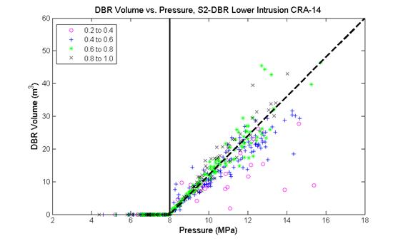
Figure PA- 75. Sensitivity of DBR Volumes to Pressure and Mobile Brine Saturation, Replicate R1, Scenario S2, Lower Intrusion, CRA-2014 PA. (Symbols indicate the range of mobile brine saturation given in the legend.)

PA-9.0 Normalized Releases

The radioactive waste disposal regulations of Part 191, Subparts B and C include containment requirements for radionuclides. The containment requirements of section 191.13 specify that releases from a disposal system to the accessible environment must not exceed the release limits set forth in 40 CFR Part 191, Appendix A, Table 1. As set forth in section 194.34, the results of PA are required to be expressed as CCDFs of total releases.

This section discusses each of the four categories of releases that constitute the total release: cuttings and cavings, spallings, DBRs, and transport releases, followed by the total normalized releases for the CRA-2014 PA. A comparison between the CRA-2014 PA and the CRA-2009 PABC results is also presented. In summary, despite the changes and corrections made between the CRA-2009 PABC and the CRA-2014 PA, there were no major changes in the overall pattern of releases. Cuttings, cavings, and DBRs remain the most significant pathways for release of radioactive material to the land surface. Contributions to total releases from spallings and Culebra transport are much less significant. The resulting CCDFs of total normalized releases for the CRA-2014 PA are within the regulatory limits defined in section 191.13.

Rank regression analysis was used to evaluate the sensitivity of the normalized releases to the sampled parameters. The predicted error sum of squares (PRESS) was computed to detect over-fitting of the regression model to the data. Over-fitting can occur when the regression methodology causes the fit to favor specific points rather than the general shape of the data curve. In such a case the minimum value of PRESS may occur earlier than the last step in the regression analysis. No such condition was observed in any of the rank correlation analyses performed in the CRA-2014 PA. Details of the sensitivity analysis performed in the CRA-2014 PA can be found in Kirchner (Kirchner 2013b).

PA-9.1 Cuttings and Cavings

The overall mean CCDFs for cuttings and cavings releases from the CRA-2014 PA and the CRA-2009 PABC are shown in Figure PA-76. Overall, cuttings and cavings normalized releases calculated for the CRA-2014 PA are smaller than those for the CRA-2009 PABC. The activity of the CRA-2014 waste inventory is greater (in EPA units) over time than that implemented in the CRA-2009 PABC (Kicker and Zeitler 2013a). The drilling rate per unit area is also increased in the CRA-2014 PA, which increases the number of drilling events into repository waste areas. Although the changes in waste inventory and drilling rate both serve to increase cuttings and cavings releases, the effect of the CRA-2014 PA waste shear strength refinement is to reduce cavings release volumes, and hence cuttings and cavings volumes overall (Kicker 2013), enough so that normalized releases due to cuttings and cavings in the CRA-2014 PA fall below those seen in the CRA-2009 PABC (Zeitler 2013).

The uncertainty in mean cuttings and cavings releases is primarily due to the uncertainty in the cuttings and cavings volume. Cuttings volume is controlled by the drill bit diameter whereas cavings volume depends on waste shear strength and, to a much smaller extent, the angular velocity of the drill string (Kicker 2013). The rank regression analysis showed that waste shear strength (BOREHOLE:TAUFAIL) controls about 65% of the variability in mean cuttings and cavings releases in replicate 1 of the CRA-2014 PA, as compared to 98% in replicate 1 of the CRA-2009 PABC. This difference is undoubtedly due to the change in the distribution of BOREHOLE:TAUFAIL from a loguniform distribution to a uniform distribution of somewhat smaller range (Kirchner 2013b).

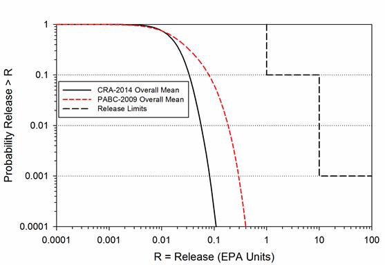
Figure PA- 76. Overall Mean CCDFs for Cuttings and Cavings Releases: CRA-2014 PA and CRA-2009 PABC

PA-9.2 Spallings

Figure PA-77 shows the overall mean spallings release CCDFs from the CRA-2014 PA and the CRA-2009 PABC. Spallings release volumes directly depend on repository pressure at the time of intrusion. Despite the modified panel closure system, which serves to increase waste panel pressures (on average), the updated steel corrosion rate, additional excavation in the WIPP experimental area, and the updated repository water balance implementation each contribute to a trend toward decreased waste panel pressures in the CRA-2014 PA. This trend toward lower waste panel pressure directly translates to a trend toward decreased spallings release volumes from the PABC-2009 to the CRA-2014 PA (Kicker 2013). The result is an overall reduction in spallings normalized releases, despite an increase in waste inventory activity, due to a decrease in the number of nonzero spallings volumes (Zeitler 2013).

The rank regression analysis indicates that the dominant uncertain parameters with regard to the uncertainty in spallings releases in the CRA-2014 PA include the particle diameter for disaggregated waste (SPALLMOD:PARTDIAM) and the initial brine pressure in the Castile

(CASTILER:PRESSURE). The intial brine pressure in the Castile impacts waste region pressures following E1 drilling intrusions which, in turn, impacts spallings release volumes and their frequency. Waste fluidization during a drilling intrusion is a function of waste particle diameter. The dominant uncertain parameter with regard to the uncertainty in spallings releases in the CRA-2009 PABC was the effective porosity of intact halite (S_HALITE:POROSITY). The number of vectors with zero spallings release volumes in the CRA-2014 PA was high enough to reduce the effectiveness of the regression analysis. A large number of zero values in the data tend to negate the assumption of linear regression that errors (residuals) are normally distributed. In addition, the distribution of zeros along the independent axis can exert a lot of influence on the slope of the regression model (Kirchner 2013b).

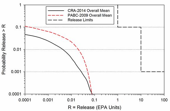
Figure PA- 77. Overall Mean CCDFs for Spallings Releases: CRA-2014 PA and CRA 2009 PABC

PA-9.3 Direct Brine

The overall mean CCDFs for DBRs from the CRA-2014 PA and the CRA-2009 PABC are shown in Figure PA-78. Overall, there is a decrease in normalized DBRs from the CRA-2009 PABC to the CRA-2014 PA. Several changes included in the CRA-2014 PA contribute to this reduction. The refinement to the probability that a drilling intrusion results in a pressurized brine pocket encounter (parameter GLOBAL:PBRINE) yields an overall reduction to DBR volumes in the CRA-2014 PA CCDFGF results (Zeitler 2013). The variable brine volume implementation maps radionuclide mobilized concentrations in brine to volumes of brine released. Radionuclide mobilized concentrations in brine decrease for the +III actinides as brine volume increases in the CRA-2014 PA (see Section PA-8.4.1), whereas mobilized concentrations in brine remained fixed (for each vector) in the CRA-2009 PABC, regardless of the actual brine volume being released. There is a consistent increase in maximum DBR volumes from the CRA-2009 PABC to the CRA-2014 PA (see Section PA-8.5.3 ). However, the variable brine volume implementation results in overall lower mobilized radionuclide concentrations in these larger brine volumes. The revised steel corrosion rate and water balance implementation used in the CRA-2014 PA also lead to an overall reduction in the number of vectors that satisfy the two necessary conditions for a DBR. In total, the combined impact of changes included in the CRA-2014 PA is an overall net reduction to normalized direct brine releases as compared to the CRA-2009 PABC.

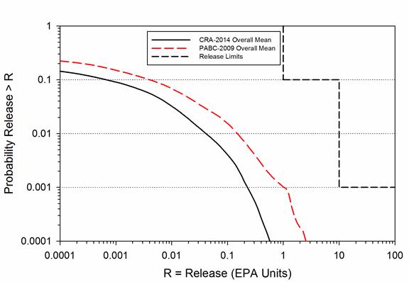
Figure PA- 78. Overall Mean CCDFs for DBRs: CRA-2014 PA and CRA-2009 PABC

The CRA-2009 PABC analysis showed that four variables (SOLMOD3:SOLVAR, CASTILER:PRESSURE, STEEL:CORRMCO2 and GLOBAL:PBRINE in Kicker and Herrick 2013, Table 4) accounted for more than 50% of the uncertainty in DBR. Variable SOLMOD3:SOLVAR is the WIPP PA parameter representing solubility uncertainty for radionuclides in the +III oxidation state. Quantity CASTILER:PRESSURE represents brine pressure in the Castile brine reservoir implemented in the WIPP PA. STEEL:CORRMCO2 represents the inundated corrosion rate for steel in the absence of CO ₂ . The WIPP PA parameter GLOBAL:PBRINE represents the probability that a drilling intrusion in an excavated repository area encounters pressurized brine. SOLMOD3:SOLVAR and CASTILER:PRESSURE are ranked first and second in importance, respectively, in all three replicates of the CRA-2014 PA. However, in the CRA-2014 PA STEEL:CORRMCO2 did not enter the regression model for any replicate, and GLOBAL:PBRINE entered the regression models of replicates 2 and 3 only in steps 5 and 13, respectively. This reduction in importance for GLOBAL:PBRINE and STEEL:CORRMCO2 is most likely related to the reduction in the ranges of the distributions assigned to these two parameters (Kirchner 2013b).

PA-9.4 Groundwater Transport

Figure PA-79 shows the mean CCDFs for normalized releases due to transport through the Culebra for the CRA-2014 PA and the CRA-2009 PABC. As seen in that figure, mean releases from the Culebra decrease from the CRA-2009 PABC to the CRA-2014 PA. Relatively few vectors (roughly 10%) contribute to nonzero Culebra transport releases (Zeitler 2013). The upper limit of the distribution for parameter GLOBAL:PBRINE has decreased from the CRA-2009 PABC to the CRA-2014 PA while the lower limit has increased. As discussed for the radionuclide transport results of Section PA-8.4.3, radionuclide transport releases to the Culebra are most likely to occur during an E1 intrusion. The refinement of the PBRINE distribution, which sets the probability that an E1 drilling intrusion occurs in a given future, results in increased Culebra transport releases for some vectors (as the PBRINE lower limit has increased) and decreases in others (as the PBRINE upper limit has decreased). The net effect is a reduction in the mean CCDF for normalized Culebra transport releases in the CRA-2014 PA as compared to the CRA-2009 PABC.

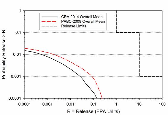
Figure PA- 79. Mean CCDFs for Releases from the Culebra: CRA-2014 PA and CRA-2009 PABC

Zero Culebra transport releases are due, for the most part, to transport rates frequently being too small to enable contaminants to reach the LWB within the 10,000-year regulatory period. The times of the intrusions giving rise to flows to the Culebra are also likely to influence whether or not such releases occur. These times are not represented in the "sampled" input parameters and thus cannot be associated with the releases in a sensitivity analysis. Changes in the releases from the Culebra are not due to changes in the rate of transport because 1) the flow fields used in the CRA-2014 analysis are the same as those used in the CRA-2009 PABC analysis, and 2) there were no changes in the matrix distribution coefficients (K _d ) for the radionuclides, so there was no change in the retardation during transport. The increase in the drilling rate may have caused some vectors to have releases that previously had none because of having earlier intrusion times in some futures, thus providing the time needed to have the radionuclides reach the LWB. In the CRA-2009 PABC the percentages of the vectors for replicates 1, 2 and 3 having zero releases were 9%, 7% and 6% respectively. In the CRA-2014 these percentages were 5%, 6% and 2%. However, in both analyses the same 32 vectors across the three replicates had releases exceeding 0.0001 EPA units (Kirchner 2013b).

PA-9.5 Total Normalized Releases

Total normalized releases for the CRA-2014 PA are presented in this section and subsequently compared to results obtained in the CRA-2009 PABC. Total releases are calculated by totaling the releases from each release pathway: cuttings and cavings releases, spallings releases, DBRs, and transport releases (there were no undisturbed releases to contribute to total release). CRA-2014 PA CCDFs for total releases obtained in replicates 1, 2, and 3 are plotted together in Figure PA-80.

The overall mean CCDF is computed as the arithmetic mean of the mean CCDFs from each replicate. To quantitatively determine the sufficiency of the sample size, a confidence interval is computed about the overall mean CCDF using the Student's t-distribution and the mean CCDFs from each replicate. Figure PA-81 shows 95% confidence intervals about the overall mean. The CCDF and confidence intervals lie below and to the left of the limits specified in section 191.13(a). Thus, the WIPP continues to comply with the containment requirements of Part 191.

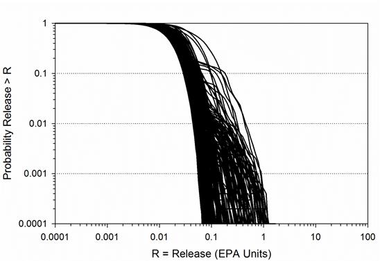
Figure PA- 80. Total Normalized Releases, Replicates R1, R2, and R3, CRA-2014 PA

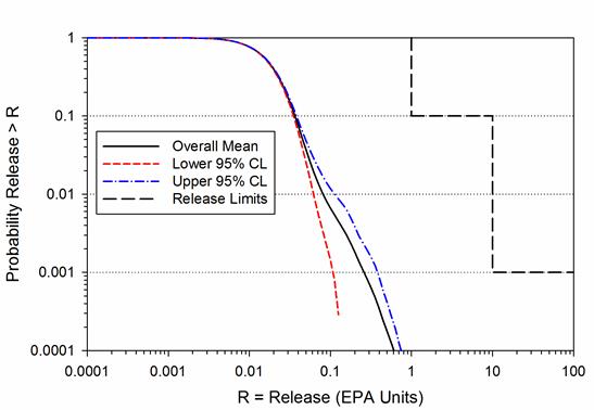
Figure PA- 81. Confidence Interval on Overall Mean CCDF for Total Normalized Releases, CRA-2014 PA

Mean CCDFs of the individual release mechanisms that comprise total normalized releases are plotted together in Figure PA-82, as well as the CRA-2014 PA total release overall mean. As seen in that figure, total normalized releases obtained in the CRA-2014 PA are dominated by cuttings and cavings releases and DBRs. Contributions to total releases from spallings and Culebra transport are much less significant. The rank regression analysis shows that the waste shear strength is the leading uncertain parameter associated with cuttings and cavings releases, and controls about 65% of mean cuttings and cavings releases in the CRA-2014 PA (Kirchner 2013b). For DBRs, the rank regression analysis shows that the solubility multiplier that represents uncertainty in solubility limits for all actinides in the III oxidation state (parameter SOLMOD3:SOLVAR) is ranked first in importance (Kirchner 2013b). The dominant release mechanisms of the CRA-2014 PA are consistent with those found in the CRA-2009 PABC, as are the leading uncertain parameters associated with those mechanisms.

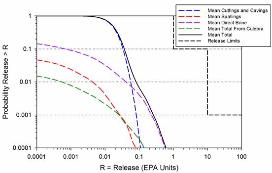
Figure PA- 82. Comparison of Overall Means for Release Componenets of the
CRA-2014 PA

Overall means for total normalized releases obtained in the CRA-2009 PABC and the CRA-2014 PA are plotted together in Figure PA-83. Overall, total normalized releases decrease from the CRA-2009 PABC to the CRA-2014 PA as each contributing component is reduced in the CRA-2014 PA.

A comparison of the statistics on the overall mean for total normalized releases obtained in the CRA-2009 PABC and the CRA-2014 PA can be seen in Table PA-29. At probabilities of 0.1 and 0.001, values obtained for the mean total release are lower for the CRA-2014 PA.

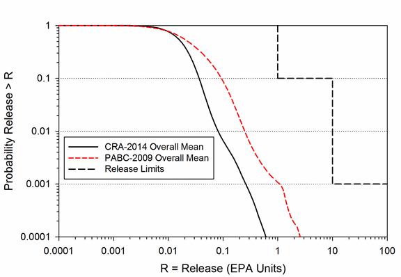
Figure PA- 83. CRA-2014 PA and CRA-2009 PABC Overall Mean CCDFs for Total Normalized Releases

Table PA- 29. CRA-2014 PA and CRA-2009 PABC Statistics on the Overall Mean for Total Normalized Releases in EPA Units at Probabilities of 0.1 and 0.001

Probability	Analysis	Mean Total Release	Lower 95% CL	Upper 95% CL	Release Limit
0.1	CRA-2014 PA	0.0367	0.0352	0.0384	1
0.1	CRA-2009 PABC	0.0937	0.0908	0.0959	1
0.001	CRA-2014 PA	0.261	0.109	0.384	10
0.001	CRA-2009 PABC	1.10	0.372	1.77	10

PA-10.0 References

(*Indicates a reference that has not been previously submitted.)

Abdul Khader, M.H., and H.S. Rao. 1974. "Flow Through Annulus with Large Radial Clearance." American Society of Civil Engineers, Journal of the Hydraulics Division, vol. 100, no. HY1: 25-39. [Author]

Antoun, T., L. Seanman, D.R. Curran, G.I. Kanel, S.V. Razorenor, and A.V. Utkin. 2003. Spall Fracture. New York: Springer-Verlag. [Author]

Aronson, D.G. 1986. The Porous Medium Equation. Nonlinear Diffusion Problems. Lecture Notes in Mathematics 1224. New York: Springer-Verlag. [Author]

Aziz, K., and A. Settari. 1979. Petroleum Reservoir Simulation. New York: Elsevier. [Author]

Barree, R.D., and M.W. Conway. 1995. "Experimental and Numerical Modeling of Convective Proppant Transport." Journal of Petroleum Technology, vol. 47 (March): 216-22. [Author]

Bateman, H. 1910. "The Solution of a System of Differential Equations Occurring in the Theory of Radio-Active Transformations." Proceedings of the Cambridge Philosophical Society, vol. 15: 423-27. [Author]

Bean, J.E., M.E. Lord, D.A. McArthur, R.J. MacKinnon, J.D. Miller, and J.D. Schreiber. 1996. Analysis Package for the Salado Flow Calculations (Task 1) of the Performance Assessment Analysis Supporting the Compliance Certification Application (CCA). ERMS 420238. Albuquerque, NM: Sandia National Laboratories. (EPA Air Docket A-93-02, Item II-G-08). [PDF / Author]

Bear, J. 1972. Dynamics of Fluids in Porous Media. New York: Dover. [Author]

Beauheim, R.L. 2003. AP-100 Task 1: Development and Application of Acceptance Criteria for Culebra Transmissivity (T) Fields, Analysis Report. ERMS 531136. Carlsbad, NM: Sandia National Laboratories. [PDF / Author]

Belhaj, H.A., K.R. Agha, A.M. Nouri, S.D. Butt, H.F. Vaziri, and M.R. Islam. 2003. Numerical Simulation of Non-Darcy Flow Utilizing the New Forchheimer's Diffusivity Equation. SPE 81499. Paper presented at the SPE 13th Middle East Oil Show & Conference, Bahrain, April 2003. [Author]

Berglund, J.W. 1992. Mechanisms Governing the Direct Removal of Wastes from the Waste Isolation Pilot Plant Repository Caused by Exploratory Drilling. SAND92-7295. Albuquerque, NM: Sandia National Laboratories. [PDF / Author]

Berglund, J.W. 1996. Analysis Package for the Cuttings and Spallings Calculations (Task 5 and 6) of the Performance Assessment Calculation Supporting the Compliance Certification Application (CCA), AP-015 and AP-016. ERMS 240521. Albuquerque, NM: Sandia National Laboratories. [PDF / Author]

Bilgen, E., R. Boulos, and A.C. Akgungor. 1973. "Leakage and Frictional Characteristics of Turbulent Helical Flow In Fine Clearance." Journal of Fluids Engineering, Transactions of the ASME, Series I, vol. 95: 493-97. [Author]

Brill, J.P., and H.D. Beggs. 1986. Two-Phase Flow in Pipes. 5th ed. Tulsa: University of Tulsa. [Author]

Brooks, R.H., and A.T. Corey. 1964. Hydraulic Properties of Porous Media. Hydrology Paper No. 3. ERMS 241117. Fort Collins, CO: Colorado State University. [PDF / Author]

Brush, L.H. and P. Domski. 2013a. Calculation of Organic-Ligand Concentrations for the WIPP CRA-2014 PA. ERMS 559005. Carlsbad, NM: Sandia National Laboratories.* [PDF / Author]

Brush, L.H. and P. Domski. 2013b. Prediction of Baseline Actinide Solubilities for the WIPP CRA-2014 PA. ERMS 559138. Carlsbad, NM: Sandia National Laboratories.* [PDF / Author]

Brush, L.H. and P. Domski. 2013c. Uncertainty Analysis of Actinide Solubilities for the WIPP CRA-2014 PA, Revision 1. ERMS 559712. Carlsbad, NM: Sandia National Laboratories.* [PDF / Author]

Bynum, R.V., C. Stockman, Y. Wang, A. Peterson, J. Krumhansl, J. Nowak, J. Cotton, M.S.Y. Chu, and S.J. Patchett. 1997. "Implementation of Chemical Controls Through a Backfill System for the Waste Isolation Pilot Plant (WIPP)." SAND96-2656C. Proceedings of the Sixth International Conference on Radioactive Waste Management and Environmental Remediation, ICEM '97, Singapore, October 12-16, 1997 (pp. 357-61). Eds. R. Baker, S. Slate, and G. Benda. New York: American Society of Mechanical Engineers. [Author]

Camphouse, R. 2013a. Design Document Criteria and Design Document for BRAGFLO, Version 6.02. ERMS 558660. Carlsbad, NM: Sandia National Laboratories.* [PDF / Author]

Camphouse, R. 2013b. Users Manual Criteria and User's Manual for BRAGFLO, Version 6.02. ERMS 558663. Carlsbad, NM: Sandia National Laboratories.* [PDF / Author]

Camphouse, R. 2013c. Analysis Package for Salado Flow Modeling Done in the 2014 Compliance Recertification Application Performance Assessment (CRA-2014 PA). ERMS 559980. Carlsbad, NM: Sandia National Laboratories.* [PDF / Author]

Camphouse, R. 2013d. Analysis Plan for the 2014 WIPP Compliance Recertification Application Performance Assessment. ERMS 559198. Carlsbad, NM: Sandia National Laboratories.* [PDF / Author]

Camphouse, R.C., D.C. Kicker, T.B. Kirchner, J.J. Long, and J.J. Pasch. 2011. Impact Assessment of SDI Excavation on Long-Term WIPP Performance. ERMS 555824. Carlsbad, NM: Sandia National Laboratories.* [PDF / Author]

Camphouse, R.C., D. Kicker, T. Kirchner, J. Long, B. Malama, and T. Zeitler. 2012a. Summary Report and Run Control for the 2012 WIPP Panel Closure System Performance Assessment. ERMS 558365. Carlsbad, NM: Sandia National Laboratories.* [PDF / Author]

Camphouse, R.C., M. Gross, C. Herrick, D. Kicker, and B. Thompson. 2012b. Recommendations and Justifications of Parameter Values for the Run-of-Mine Salt Panel Closure System Design Modeled in the PCS-2012 PA. Memo to WIPP Records Center dated May 3, 2012. ERMS 557396. Carlsbad, NM: Sandia National Laboratories.* [PDF / Author]

Camphouse, R., D. Kicker, S. Kim, T. Kirchner, J. Long, B. Malama, T. Zeitler. 2013. Summary Report for the 2014 WIPP Compliance Recertification Application Performance Assessment. ERMS 560252. Carlsbad, NM: Sandia National Laboratories.* [PDF / Author]

Caporuscio, F., J. Gibbons, and E. Oswald. 2003. Waste Isolation Pilot Plant: Salado Flow Conceptual Models Final Peer Review Report. ERMS 526879. Carlsbad, NM: Carlsbad Area Office, Office of Regulatory Compliance. [PDF / Author]

Carlsbad Area Office Technical Assistance Contractor (CTAC). 1997. Expert Elicitation on WIPP Waste Particle-Size Distribution(s) During the 10,000-Year Regulatory Post-Closure Period (Final Report, June 3). ERMS 541365. Carlsbad, NM: U.S. Department of Energy. [PDF / Author]

Chambre Syndicale de la Recherche et de la Production du Petrole et du Gaz Naturel. 1982. Drilling Mud and Cement Slurry Rheology Manual. English translation. Houston: Gulf Publishing. [Author]

Chappelear, J.E., and A.S. Williamson. 1981. "Representing Wells in Numerical Reservoir Simulation: Part 2-Implementation." Society of Petroleum Engineers Journal, vol. 21: 339-44. [Author]

Cherimisinoff, N.P., and P.N. Cherimisinoff. 1984. Hydrodynamics of Gas-Solids Fluidization. Houston, TX: Gulf Publishing. [Author]

Christian-Frear, T.L. 1996. Salado Halite Permeability from Room Q Analysis. ERMS 414996. Albuquerque, NM: Sandia National Laboratories. [PDF / Author]

Clayton, D.J. 2007. Corrections to Input Files for DBR PABC Calculations. ERMS 546311. Carlsbad, NM: Sandia National Laboratories. [PDF / Author]

Clayton, D.J. 2008a. Analysis Plan for the Performance Assessment for the 2009 Compliance Recertification Application (Revision 1). AP-137. ERMS 547905. Carlsbad, NM: Sandia National Laboratories. [PDF / Author]

Clayton, D.J. 2008b. Memorandum to L. Brush (Subject: Update to the Calculation of the Minimum Brine Volume for a Direct Brine Release). 2 April 2008. ERMS 548522. Carlsbad, NM: Sandia National Laboratories.* [PDF / Author]

Clayton, D.J. 2009. Update to Kd Values for the PABC-2009. ERMS 552395. Carlsbad, NM: Sandia National Laboratories.* [PDF / Author]

Clayton, D.J. 2013. Justification of Chemistry Parameters for Use in BRAGFLO for AP-164, Revision 1. ERMS 559466. Carlsbad, NM: Sandia National Laboratories.* [PDF / Author]

Clayton, D.J., S. Dunagan, J.W. Garner, A.E. Ismail, T.B. Kirchner, G.R. Kirkes, and M.B. Nemer. 2008. Summary Report of the 2009 Compliance Recertification Application Performance Assessment. ERMS 548862. Carlsbad, NM: Sandia National Laboratories. [PDF / Author]

Clayton, D.J., R.C. Camphouse, J.W. Garner, A.E. Ismail, T.B. Kirchner, K.L. Kuhlman, M.B. Nemer. 2010. Summary Report of the CRA-2009 Performance Assessment Baseline Calculation. ERMS 553039. Carlsbad, NM: Sandia National Laboratories.* [PDF / Author]

Corbet, T.F., and P.M. Knupp. 1996. The Role of Regional Groundwater Flow in the Hydrogeology of the Culebra Member of the Rustler Formation at the Waste Isolation Pilot Plant (WIPP), Southeastern New Mexico. SAND96-2133. Albuquerque, NM: Sandia National Laboratories. [PDF / Author]

Corbet, T., and P. Swift. 1996a. Memorandum to M.S. Tierney (Subject: Distribution for Non-Salado Parameter for SECOFL2D: Climate Index). 12 April 1996. ERMS 237465. Albuquerque, NM: Sandia National Laboratories. [PDF / Author]

Corbet, T., and P. Swift. 1996b. Parameters Required for SECOFL2D: Climate Index. Record Package. ERMS 237465. Albuquerque, NM: Sandia National Laboratories. [PDF / Author]

Cotsworth, E. 2005. Letter to U.S. Department of Energy (1 Enclosure). March 4, 2005. ERMS 538858. Washington, DC: U.S. Environmental Protection Agency, Office of Air and Radiation. [PDF / Author]

Cotsworth, E. 2009. EPA Letter on CRA-2009 First Set of Completeness Comments. ERMS 551444. Washington, DC: U.S. Environmental Protection Agency, Office of Radiation and Indoor Air.* [PDF / Author]

Cranwell, R.M., R.V. Guzowski, J.E. Campbell, and N.R. Ortiz. 1990. Risk Methodology for Geologic Disposal of Radioactive Waste: Scenario Selection Procedure. NUREG/CR-1667. SAND80-1429. ERMS 226750. Albuquerque, NM: Sandia National Laboratories. [PDF / Author]

Darley, H.C.H. 1969. "A Laboratory Investigation of Borehole Stability." JPT Journal of Petroleum Technology, July: 883-92. [Author]

Doherty, J. 2002. Design Document (DD) for PEST Version 5.5. ERMS 523970. Los Alamos, NM: Los Alamos National Laboratories. [PDF / Author]

Ely, J.F., and M.L. Huber. 1992. NIST Thermophysical Properties of Hydrocarbon Mixtures Database (SUPERTRAPP), Version 1.0, User's Guide. ERMS 242589. Gaithersburg, MD: U.S. Department of Commerce, National Institute of Standards and Technology, Standard Reference Data Program. [Author]

Ergun, S. 1952. "Fluid Flow Through Packed Columns." Chemical Engineering Progress, vol. 48: 89-94. [Author]

Fletcher, C.A.J. 1988. Computational Techniques for Fluid Dynamics. 2nd ed. Vols. 1 and 2. New York: Springer-Verlag. [Author]

Fox, R.W., and A.T. McDonald. 1985. Introduction to Fluid Mechanics. 3rd ed. New York: Wiley. [Author]

Francis, A.J., J.B. Gillow, and M.R. Giles. 1997. Microbial Gas Generation Under Expected Waste Isolation Pilot Plant Repository Conditions. SAND96-2582. Albuquerque, NM: Sandia National Laboratories. [PDF / Author]

Frigaard, I.A., and N.L. Humphries. 1997. "High Penetration Rates: Hazards and Well Control-A Case Study." Proceedings, March 1997 Society of Petroleum Engineers/International Association of Drilling Contractors Drilling Conference (SPE paper 37953). Amsterdam: Society of Petroleum Engineers. [Author]

Gatlin, C. 1960. Petroleum Engineering: Drilling and Well Completions. Englewood Cliffs, NJ: Prentice-Hall. [Author]

Graboski, M.S., and T.E. Daubert. 1979. A Modified Soave Equation of State for Phase Equilibrium Calculations: 3: Systems Containing Hydrogen. Industrial and Engineering Chemistry Process Design and Development, vol. 18: 300-06. [Author]

Haberman, J.H., and D.J. Frydrych. 1988. "Corrosion Studies of A216 Grade WCA Steel in Hydrothermal Magnesium-Containing Brines." Materials Research Society Symposium Proceedings: Scientific Basis for Nuclear Waste Management XI (pp. 761-72). Eds. M.J. Apted and R.E. Westerman. Pittsburgh: Materials Research Society. [Author]

Hadgu, T., P. Vaughn, J. Bean, D. Johnson, J. Johnson, K. Aragon, and J. Helton. 1999. Memorandum to M. Marietta (Subject: Modifications to the 96 CCA Direct Brine Release Calculations). 2 November 1999. ERMS 511276. Carlsbad, NM: Sandia National Laboratories. [PDF / Author]

Hansen, F.D., M.K. Knowles, T.W. Thompson, M. Gross, J.D. McLennan, and J.F. Schatz. 1997. Description and Evaluation of a Mechanistically Based Conceptual Model for Spall. SAND97-1369. Albuquerque, NM: Sandia National Laboratories. [PDF / Author]

Hansen, F.D., T.W. Pfeifle, and D.L. Lord. 2003. Parameter Justification Report for DRSPALL. ERMS 531057. Carlsbad, NM: Sandia National Laboratories. [PDF / Author]

Harbaugh, A.W., E.R. Banta, M.C. Hill, and M.G. McDonald. 2000. MODFLOW-2000: The U.S. Geological Survey Modular Ground-Water Model-User Guide to Modularization Concepts and the Ground-Water Flow Process. Open File Report 00-92. Reston, VA: U.S. Geological Survey. [PDF / Author]

Hart, D., R. Beauheim, and S. McKenna. 2009. Analysis Report for Task 7 of AP-114: Calibration of Culebra Transmissivity Fields. ERMS 552391. Carlsbad, NM: Sandia National Laboratories.* [PDF / Author]

Helton, J.C. 1993. "Drilling Intrusion Probabilities for Use in Performance Assessment for Radioactive Waste Disposal." Reliability Engineering and System Safety, vol. 40: 259-75. [Author]

Helton, J.C., J.D. Johnson, M.D. McKay, A.W. Shiver, and J.L. Sprung. 1995. "Robustness of an Uncertainty and Sensitivity Analysis of Early Exposure Results with the MACCS Reactor Accident Consequence Model." Reliability Engineering and System Safety, vol. 48, no. 2: 129-48. [Author]

Helton, J.C., J.E. Bean, J.W. Berglund, F.J. Davis, K. Economy, J.W. Garner, J.D. Johnson, R.J. MacKinnon, J. Miller, D.G. O'Brien, J.L. Ramsey, J.D. Schreiber, A. Shinta, L.N. Smith, D.M. Stoelzel, C. Stockman, and P. Vaughn. 1998. Uncertainty and Sensitivity Analysis Results Obtained in the 1996 Performance Assessment for the Waste Isolation Pilot Plant. SAND98-0365. Albuquerque, NM: Sandia National Laboratories. [PDF / Author]

Helton, J.C., and F.J. Davis. 2003. "Latin Hypercube Sampling and the Propagation of Uncertainty in Analyses of Complex Systems." Reliability Engineering and System Safety. vol. 81, no. 1: 23-69. [Author]

Herrick, C.G., M.D. Schuhen, D.M. Chapin, and D.C. Kicker. 2012. Determining the Hydrodynamic Shear Strength of Surrogate Degraded TRU Waste Materials as an Estimate for the Lower Limit of the Performance Assessment Parameter TAUFAIL. ERMS 558479. Carlsbad, NM: Sandia National Laboratories.* [PDF / Author]

Herrick, C.G. 2013. Memorandum to C. Camphouse (Subject: Follow-up to Questions Concerning TAUFAIL Flume Testing Raised during the November 14-15, 2012 Technical Exchange Between the DOE and EPA). 23 January 2013. ERMS 559081. Carlsbad, NM: Sandia National Laboratories.* [PDF / Author]

Hirsch, C. 1988. "Numerical Computation of Internal and External Flows." Fundamentals of Numerical Discretization. Vol. 1. Chichister, UK: John Wiley & Sons. [Author]

Howard, B.A. 1996. Memorandum to Sandia National Laboratories (Subject: Performance Assessment Parameter Input). 23 February 1996. ERMS 247595. Carlsbad, NM: Westinghouse Electric Corporation. [PDF / Author]

Howarth, S.M., and T. Christian-Frear. 1997. Porosity, Single-Phase Permeability, and Capillary Pressure Data from Preliminary Laboratory Experiments on Selected Samples from Marker Bed 139 at the Waste Isolation Pilot Plant. SAND94-0472/1/2/3. Albuquerque, NM: Sandia National Laboratories. [PDF / Author]

Hunter, R.L. 1985. A Regional Water Balance for the Waste Isolation Pilot Plant (WIPP) Site and Surrounding Area. SAND84-2233. Albuquerque, NM: Sandia National Laboratories. [PDF / Author]

Huyakorn, P.S., B.H. Lester, and J.W. Mercer. 1983. "An Efficient Finite Element Technique for Modelling Transport in Fractured Porous Media: 1. Single Species Transport." Water Resources Research, vol. 19: 841-54. [Author]

Iman, R.L. 1982. "Statistical Methods for Including Uncertainties Associated with the Geologic Isolation of Radioactive Waste Which Allow for a Comparison with Licensing Criteria." Proceedings of the Symposium on Uncertainties Associated with the Regulation of the Geologic Disposal of High-Level Radioactive Waste, March 9-13, 1981 (pp. 145-57). Ed. D.C. Kocher. NUREG/CP-0022, CONF-810372. Washington, DC: U.S. Nuclear Regulatory Commission, Directorate of Technical Information and Document Control. [Author]

Iman, R.L., M.J. Shortencarier, and J.D. Johnson. 1985. A FORTRAN 77 Program and User's Guide for the Calculation of Partial Correlation and Standardized Regression Coefficients. SAND85-0044. NUREG/CR-4122. Albuquerque, NM: Sandia National Laboratories. [PDF / Author]

Iman, R.L., and W.J. Conover. 1979. "The Use of the Rank Transform in Regression." Technometrics, vol. 21: 499-509. [Author]

Iman, R.L., and W.J. Conover. 1982. "A Distribution-Free Approach to Inducing Rank Correlation Among Input Variables." Communications in Statistics: Simulation and Computation, vol. B11, no. 3: 311-34. [Author]

Iman, R.L., and J.C. Helton. 1988. "An Investigation of Uncertainty and Sensitivity Analysis Techniques for Computer Models." Risk Analysis, vol. 8: 71-90. [Author]

Iman, R.L., and J.C. Helton. 1991. "The Repeatability of Uncertainty and Sensitivity Analyses for Complex Probabilistic Risk Assessments." Risk Analysis, vol. 11: 591-606. [Author]

Jaeger, J.C. and N.G.W. Cook. 1969. Fundamentals of Rock Mechanics, Chapman and Hall Ltd., London, England.* [Author]

James, S.J., and J. Stein. 2003. Analysis Report for the Development of a Simplified Shaft Seal Model for the WIPP Performance Assessment (Rev 1). ERMS 525203. Carlsbad, NM: Sandia National Laboratories. [PDF / Author]

Kaufmann, D.W., ed. 1960. Sodium Chloride: The Production and Properties of Salt and Brine. American Chemical Society Monograph 145. New York: Reinhold. [Author]

Kelly, T. 2009. EPA Third Letter Requesting Additional Information on the CRA-2009. ERMS 552374. Washington, DC: U.S. EPA Office of Radiation and Indoor Air.* [PDF / Author]

Kicker, D. 2013. Analysis Package for Cuttings, Cavings, and Spallings: 2014 Complinace Recertification Application Performance Assessment (CRA-2014 PA). ERMS 560060. Carlsbad, NM: Sandia National Laboratories.* [PDF / Author]

Kicker, D. and C. Herrick. 2013. Parameter Summary Report for the 2014 Compliance Recertification Application. Carlsbad, NM: Sandia National Laboratories.* [PDF / Author]

Kicker, D. and and T. Zeitler. 2013a. Analysis Package for EPA Unit Loading Calculations for the 2014 Compliance Recertification Application Performance Assessment (CRA-2014 PA). ERMS 560065. Carlsbad, NM: Sandia National Laboratories.* [PDF / Author]

Kicker, D. and and T. Zeitler. 2013b. Radionuclide Inventory Screening Analysis for the 2014 Compliance Recertification Application Performance Assessment (CRA-2014 PA). ERMS 559257. Carlsbad, NM: Sandia National Laboratories.* [PDF / Author]

Kim, S. 2013a. Analysis Package for Salado Transport Calculations: CRA-2014 Performance Assessment. ERMS 560174. Carlsbad, NM: Sandia National Laboratories.* [PDF / Author]

Kim, S. 2013b. Analysis Package for PANEL: CRA-2014 Performance Assessment. ERMS 560174. Carlsbad, NM: Sandia National Laboratories. [PDF / Author]

Kim, S. and R. Camphouse. 2013. Marker Bed Concentrations and Radium-226 Concentration for Undisturbed NUTS Scenario in AP-164. Memorandum to SNL WIPP Records Center dated April 25, 2013. ERMS 559914. Carlsbad, NM: Sandia National Laboratories.* [PDF / Author]

Kirchner, T. 2013a. Generation of the LHS Samples for the CRA-2014 (AP-164) PA Calculations. ERMS 559950. Carlsbad, NM: Sandia National Laboratories.* [PDF / Author]

Kirchner, T. 2013b. Sensitivity of the CRA-2014 Performance Assessment Releases to Parameters. ERMS 560043. Carlsbad, NM: Sandia National Laboratories.* [PDF / Author]

Kirchner, T., T. Zeitler, and R. Kirkes. 2012. Evaluating the Data in Order to Derive a Value for GLOBAL:PBRINE. Memorandum to Sean Dunagan dated December 11, 2012. ERMS 558724. Carlsbad, NM: Sandia National Laboratories.* [PDF / Author]

Kirkes, R. 2007. Evaluation of the Duration of Direct Brine Release in WIPP Performance Assessment (Revision 0). ERMS 545988. Carlsbad, NM: Sandia National Laboratories. [PDF / Author]

Klinkenberg, L.J. 1941. The Permeability of Porous Media to Liquids and Gases (pp. 200-13). API Drilling and Production Practice. ERMS 208556. Albuquerque, NM: Sandia National Laboratories. [PDF / Author]

Kuhlman, K. 2010. Analysis Report for the CRA-2009 PABC Culebra Flow and Transport Calculations. ERMS 552951. Carlsbad, NM: Sandia National Laboratories.* [PDF / Author]

Lee, J. 1982. Well Testing. SPE Textbook Series Vol. 1. New York: Society of Petroleum Engineers of AIME. [Author]

Leigh, C., R. Beauheim, and J. Kanney. 2003. SNL WIPP Analysis Plan AP-100, Revision 0, Analysis Plan for Calculation of Culebra Flow and Transport, Compliance Recertification Application. ERMS 530172. Carlsbad, NM: Sandia National Laboratories. [PDF / Author]

Li, D., R.K. Svec, T.W. Engler, and R.B. Grigg. 2001. Modeling and Simulation of the Wafer Non-Darcy Flow Experiments. SPE 68822. Paper presented at the SPE Western Regional Meeting, Bakersfield, CA, March 26-30. [Author]

Lide, D.R., ed. 1991. CRC Handbook of Chemistry and Physics. 72nd ed. Boca Raton: CRC Press. [Author]

Long, J. 2013. Execution of Performance Assessment Codes for the CRA-2014 Performance Assessment. ERMS 560016. Carlsbad, NM: Sandia National Laboratories. [PDF / Author]

Lord, D.L., D.K. Rudeen, and C.W. Hansen. 2003. Analysis Package for DRSPALL: Compliance Recertification Application Part I: Calculation of Spall Volume. ERMS 532766. Carlsbad, NM: Sandia National Laboratories. [PDF / Author]

Lord, D.L., and D.K. Rudeen. 2003. Sensitivity Analysis Report: Parts I and II: DRSPALL Version 1.00: Report for Conceptual Model Peer Review July 7-11. ERMS 524400. Carlsbad, NM: Sandia National Laboratories. [PDF / Author]

Lorenz, J.C. 2006a. Assessment of the Potential for Karst in the Rustler Formation at the WIPP Site. SAND2005-7303. Albuquerque, NM: Sandia National Laboratories.* [PDF / Author]

Lorenz, J.C. 2006b. Assessment of the Geological Evidence for Karst in the Rustler Formation at the WIPP Site. Caves and Karst of Southeastern New Mexico (pp. 243-52). L. Land, V.W.* [Author]

Lowry, T. 2003. Analysis Package for Salado Transport Calculations: Compliance Recertification Application (Revision 0). ERMS 530163. Carlsbad, NM: Sandia National Laboratories. [PDF / Author]

Lowry, T.S. 2005. Analysis Package for Salado Transport Calculations: CRA-2004 PA Baseline Calculation. ERMS 541084. Carlsbad, NM: Sandia National Laboratories. [PDF / Author]

Malama, B. 2013. Analysis Package for Direct Brine Releases: CRA-2014 Performance Assessment (CRA-2014 PA). ERMS 560069. Carlsbad, NM: Sandia National Laboratories.* [PDF / Author]

Martell, M. 1996a. Memorandum to C. Lattier (Subject: Additional Information for the DRZ [Disturbed Rock Zone] Porosity). 14 November 1996. ERMS 242257. Albuquerque, NM: Sandia National Laboratories. [PDF / Author]

Martell, M. 1996b. Memorandum to C. Lattier (Subject: Additional Information for the Culebra Transport Parameter Id: 843, idpram: DNSGRAIN, idmtrl: CULEBRA, WIPP Data Entry Form 464 at WPO # 32689). 10 December 1996. ERMS 232689. Albuquerque, NM: Sandia National Laboratories. [PDF / Author]

Mattax, C.C., and R.L. Dalton. 1990. Reservoir Simulation. SPE Monograph 13. Richardson, TX: Henry L. Doherty Memorial Fund of Society of Petroleum Engineers, Inc. [Author]

McDonald, M.G., and A.W. Harbaugh. 1988. "A Modular Three-Dimensional Finite-Difference Ground-Water Flow Model." U.S. Geological Survey Techniques of Water-Resources Investigations. Book 6, Chap. A1. U.S. Government Printing Office. [Author]

McKay, M.D., R.J. Beckman, and W.J. Conover. 1979. "A Comparison of Three Methods for Selecting Values of Input Variables in the Analysis of Output from a Computer Code." Technometrics, vol. 21: 239-45. [Author]

McKenna, S.A., and D.B. Hart. 2003. Analysis Report: Task 4 of AP-088 Conditioning of Base T-Fields to Transient Heads. ERMS 531124. Albuquerque, NM: Sandia National Laboratories. [PDF / Author]

McTigue, D.F. 1993. Permeability and Hydraulic Diffusivity of Waste Isolation Pilot Plant Repository Salt Inferred from Small-Scale Brine Inflow Experiments. SAND92-1911. Albuquerque, NM: Sandia National Laboratories. [PDF / Author]

Meigs, L. 1996. Memorandum to J. Ramsey (Subject: Non-Salado: Diffusive Tortuosity for the Culebra Dolomite). 16 May 1996. ERMS 238940. Albuquerque, NM: Sandia National Laboratories. [PDF / Author]

Meigs, L., and J. McCord. 1996. Physical Transport in the Culebra Dolomite. ERMS 239167. Albuquerque, NM: Sandia National Laboratories. [PDF / Author]

Meigs, L., R.L. Beauheim, and T.L. Jones (eds). 2000. Interpretations of Tracer Tests Performed in the Culebra Dolomite at the Waste Isolation Pilot Plant Site. SAND97-3109. Albuquerque, NM: Sandia National Laboratories. [PDF / Author]

Mendenhall, F.T., and W. Gerstle. 1995. WIPP Anhydrite Fracture Modeling, Systems Prioritization Method - Iteration 2 Baseline Position Paper: Disposal Room and Cutting Models. ERMS 239830. Albuquerque, NM: Sandia National Laboratories. [PDF / Author]

Myers, R.H. 1986. Classical and Modern Regression with Applications. Boston: Duxbury. [Author]

Nemer, M.B. 2007. Effects of Not Including Emplacement Materials in CPR Inventory on Recent PA Results. ERMS 545689. Carlsbad, NM: Sandia National Laboratories. [PDF / Author]

Nemer, M.B., and D.J. Clayton. 2008. Analysis Package for Salado Flow Modeling, 2009 Compliance Recertification Application Calculation. ERMS 548607. Carlsbad, NM: Sandia National Laboratories. [PDF / Author]

Nemer, M.B., and J.S. Stein. 2005. Analysis Package for BRAGFLO, 2004 Compliance Recertification Application Performance Assessment Baseline Calculation (June 28). ERMS 540527. Carlsbad, NM: Sandia National Laboratories. [PDF / Author]

Nemer, M.B., J.S. Stein, and W. Zelinski. 2005. Analysis Report for BRAGFLO Preliminary Modeling Results With New Gas Generation Rates Based Upon Recent Experimental Results. ERMS 539437. Carlsbad, NM: Sandia National Laboratories. [PDF / Author]

Nemer, M.B. and W. Zelinski. 2005. Analysis Report for BRAGFLO Modeling Results with the removal of Methanogenesis from the Microbial-Gas-Generation Model. ERMS 538748. Carlsbad, NM: Sandia National Laboratories. [PDF / Author]

Oldroyd, J.G. 1958. "Non-Newtonian Effects in Steady Motion of Some Idealized Elastico-Viscous Liquids." Proceedings of the Royal Society of London: Series A: Mathematical and Physical Sciences, vol. 245, no. 1241: 278-97. ERMS 243211. [Author]

Papenguth, H.W. 1996. Parameter Record Package for Colloid Actinide Retardation Parameters. WPO 38173, Sandia WIPP Central Files (SWCF). [PDF / Author]

Peake, Thomas. 1998. Technical Report Review of TDEM Analysis of WIPP Brine Pockets. Washington, DC: U. S. Environmental Protection Agency, Office of Radiation and Indoor Air.* [PDF / Author]

Podio, A.L., and A.P. Yang. 1986. Well Control Simulator for IBM Personal Computer. IADC/SPE 14737. Paper presented at the International Association of Drilling Engineers/Society of Petroleum Engineers Drilling Conference. Dallas, TX, February 10-12. [Author]

Poettmann, F.H., and P.G. Carpenter. 1952. "Multiphase Flow of Gas, Oil, and Water Through Vertical Flow Strings with Application to the Design of Gas-lift Installations." Drilling and Production Practice (1952): 257-317. [Author]

Popielak, R.S., R.L. Beauheim, S.R. Black, W.E. Coons, C.T. Ellingson, and R.L. Olsen. 1983. Brine Reservoirs in the Castile Formation Waste Isolation Pilot Plant (WIPP) Project Southeastern New Mexico. TME-3153. Carlsbad, NM: Westinghouse Electric Corp. [PDF / Author]

Prasuhn, A.L. 1980. Fundamentals of Fluid Mechanics. Englewood Cliffs, NJ: Prentice-Hall. [Author]

Prausnitz, J.M. 1969. Molecular Thermodynamics of Fluid-Phase Equilibria. Englewood Cliffs, NJ: Prentice-Hall. [Author]

Press, W.H., B.P. Flannery, S.A. Teukolsky, and W.T. Vetterling. 1989. Numerical Recipes in Pascal: The Art of Scientific Computing. Cambridge: Cambridge U P. [Author]

Rechard, R. P., A. C. Peterson, J. D. Schreiber, H. J. Iuzzolino, M. S. Tierney and J. S. Sandha. 1991. Preliminary comparison with 40 CFR Part 191, Subpart B for the Waste Isolation Pilot Plant, December 1991; Volume 3: Reference Data. Albuquerque, NM: Sandia National Laboratories.* [PDF / Author]

Rechard, R.P., H. Iuzzolino, and J.S. Sandha. 1990. Data Used in Preliminary Performance Assessment of the Waste Isolation Pilot Plant (1990). SAND89-2408. Albuquerque, NM: Sandia National Laboratories. [PDF / Author]

Reed, D.J., J. Swanson, J.-F. Lucchini and M. Richman. 2013. Intrinsic, Mineral and Microbial Colloid Enhancement Parameters for the WIPP Actinide Source Term. ERMS 559200. LCO-ACP-18. Carlsbad, NM: Los Alamos Laboratory.* [PDF / Author]

Roberts, R. 1996. Salado: Brine Compressibility. Records Package. ERMS 412842. Albuquerque, NM: Sandia National Laboratories. [PDF / Author]

Roselle, G.T. 2013. Determination of Corrosion Rates from Iron/Lead Corrosion Experiments to be used for Gas Generation Calculations. ERMS 559077. Carlsbad, NM: Sandia National Laboratories.* [PDF / Author]

Ross, S.M. 1987. Introduction to Probability and Statistics for Engineers and Scientists. New York: John Wiley & Sons. [Author]

Ruth, D., and H. Ma. 1992. "On the Derivation of the Forchheimer Equation by Means of the Averaging Theorem." Transport in Porous Media, vol. 7: 255-64. [Author]

Sallaberry, C.J., J.C. Helton, and S.C. Hora. 2006. Extension of Latin Hypercube Samples with Correlated Variables. SAND2006-6135. Albuquerque, NM: Sandia National Laboratories. [PDF / Author]

Sandia National Laboratories (SNL). 1992. Preliminary Performance Assessment for the Waste Isolation Pilot Plant, December 1992. 5 vols. SAND92-0700/1-5. Albuquerque, NM: Sandia National Laboratories. [PDF / Author]

Sandia National Laboratories (SNL). 1997. Summary of Uncertainty and Sensitivity Analysis Results for the EPA-Mandated Performance Assessment Verification Test. ERMS 420667. Albuquerque, NM: Sandia National Laboratories. [PDF / Author]

Savins, J.G., and G.C. Wallick. 1966. "Viscosity Profiles, Discharge Rates, Pressures, and Torques for a Rheologically Complex Fluid in a Helical Flow." A.I.Ch.E. Journal, vol. 12: 357-63. [Author]

Stein, J.S. 2002. Memorandum to M.K. Knowles (Subject: Methodology behind the TBM BRAGFLO Grid), 13 May 2002. ERMS 522373. Carlsbad, NM: Sandia National Laboratories. [PDF / Author]

Stein, J.S. and W. Zelinski. 2003. Analysis Report for: Testing of a Proposed BRAGFLO Grid to be used for the Compliance Recertification Application Performance Assessment Calculations. ERMS 526868. Carlsbad, NM: Sandia National Laboratories. [PDF / Author]

Stockman, C., A. Shinta, and J. Garner, J. 1996. Analysis Package for the Salado Transport Calculations (Task 2) of the Performance Assessment Analysis Supporting the Compliance Certification Application. ERMS 422314. Carlsbad, NM: Sandia National Laboratories. [PDF / Author]

Stoelzel, D.M., and D.G. O'Brien. 1996. Analysis Package for the BRAGFLO Direct Release Calculations (Task 4) of the Performance Assessment Calculations Supporting the Compliance Certification Application (CCA), AP-029, Brine Release Calculations. ERMS 240520. Albuquerque, NM: Sandia National Laboratories. [PDF / Author]

Stone, C.M. 1997. SANTOS-A Two-Dimensional Finite Element Program for the Quasistatic, Large Deformation, Inelastic Response of Solids. SAND90-0543. Albuquerque, NM: Sandia National Laboratories. [PDF / Author]

Streeter, V.L. 1958. Fluid Mechanics. 2nd ed. New York: McGraw-Hill. [Author]

Sweby, P.K. 1984. "High Resolution Schemes Using Flux Limiters for Hyperbolic Conservation Laws." SIAM Journal on Numerical Analysis, vol. 21: 995-1011. [Author]

Telander, M.R., and R.E. Westerman. 1993. Hydrogen Generation by Metal Corrosion in Simulated Waste Isolation Pilot Plant Environments: Progress Report for the Period November 1989 Through December 1992. SAND92-7347. Albuquerque, NM: Sandia National Laboratories. [PDF / Author]

Telander, M.R., and R.E. Westerman. 1997. Hydrogen Generation by Metal Corrosion in Simulated Waste Isolation Pilot Plant Environments. SAND96-2538. Albuquerque, NM: Sandia National Laboratories. [PDF / Author]

Thompson, T.W., W.E. Coons, J.L. Krumhansl, and F.D. Hansen. 1996. Inadvertent Intrusion Borehole Permeability (July). ERMS 241131. Albuquerque, NM: Sandia National Laboratories. [PDF / Author]

Tierney, M.S. 1990. Constructing Probability Distributions of Uncertain Variables in Models of the Performance of the Waste Isolation Pilot Plant: the 1990 Performance Simulations. SAND 90-2510. Albuquerque, NM: Sandia National Laboratories. [PDF / Author]

Timoshenko, S.P., and J.N. Goodier. 1970. Theory of Elasticity. 3rd ed. New York: McGraw-Hill. [Author]

Trovato, E.R. 1997. Letter to A. Alm (6 Enclosures). 19 March 1997. ERMS 245835. Washington, DC: U.S. Environmental Protection Agency, Office of Air and Radiation. [PDF / Author]

U.S. Department of Energy (DOE). 1995. Waste Isolation Plant Sealing System Design Report. DOE/WIPP-95-3117. Carlsbad, NM: U.S. Department of Energy, Carlsbad Area Office. [PDF / Author]

U.S. Department of Energy (DOE). 1996. Title 40 CFR Part 191 Compliance Certification Application for the Waste Isolation Pilot Plant (October). 21 vols. DOE/CAO 1996-2184. Carlsbad, NM: U.S. Department of Energy, Carlsbad Area Office. [Author]

U.S. Department of Energy (DOE). 1997. Supplemental Summary of EPA-Mandated Performance Assessment Verification Test (All Replicates) and Comparison with the Compliance Certification Application Calculations (August 8). WPO 46702. ERMS 414879. Carlsbad, NM: U.S. Department of Energy, Carlsbad Area Office. [PDF / Author]

U.S. Department of Energy (DOE). 2004. Title 40 CFR Part 191 Compliance Recertification Application for the Waste Isolation Pilot Plant (March). 10 vols. DOE/WIPP 2004-3231. Carlsbad, NM: U.S. Department of Energy, Carlsbad Field Office. [Author]

U.S. Department of Energy (DOE). 2009. Title 40 CFR Part 191 Compliance Recertification Application for the Waste Isolation Pilot Plant. DOE/WIPP 09-3424. Carlsbad, NM: U.S. Department of Energy, Carlsbad Field Office. [Author]

U.S. Department of Energy (DOE). 2011a. Panel Closure System Design, Planned Change Request to the EPA 40 CFR Part 194 Certification of the Waste Isolation Pilot Plant. Carlsbad, NM: U.S. Department of Energy, Carlsbad Field Office.* [PDF / Author]

U.S. Department of Energy (DOE). 2011b. Letter from E. Ziemianski to J. Edwards (Subject: Notification of Intent to Begin the Salt Disposal Investigations). 11 August 2011. Carlsbad, NM: U.S. Department of Energy, Carlsbad Field Office.* [PDF / Author]

U.S. Department of Energy (DOE). 2012. Delaware Basin Monitoring Annual Report. DOE/WIPP-12-2308. Carlsbad, NM: Carlsbad Field Office.* [PDF / Author]

U.S. Environmental Protection Agency (EPA). 1985. 40 CFR 191: Environmental Standards for the Management and Disposal of Spent Nuclear Fuel, High-Level and Transuranic Radioactive Wastes; Final Rule. Federal Register, vol. 50 (September 19, 1985): 38066-089. [PDF / Author]

U.S. Environmental Protection Agency (EPA). 1993. "40 CFR 191: Environmental Radiation Protection Standards for the Management and Disposal of Spent Nuclear Fuel, High-Level and Transuranic Radioactive Wastes; Final Rule." Federal Register, vol. 58 (December 20, 1993): 66398-416. [PDF / Author]

U.S. Environmental Protection Agency (EPA). 1996a. "40 CFR Part 194: Criteria for the Certification and Recertification of the Waste Isolation Pilot Plant's Compliance with the 40 CFR Part 191 Disposal Regulations; Final Rule." Federal Register, vol. 61 (February 9, 1996): 5223-45. [PDF / Author]

U.S. Environmental Protection Agency (EPA). 1996b. Background Information Document for 40 CFR Part 194 (January). EPA 402-R-96-002. Washington, DC: Office of Radiation and Indoor Air. [PDF / Author]

U.S. Environmental Protection Agency (EPA). 1998a. "40 CFR Part 194: Criteria for the Certification and Recertification of the Waste Isolation Pilot Plant's Compliance with the Disposal Regulations: Certification Decision; Final Rule." Federal Register, vol. 63 (May 18, 1998): 27353-406. [PDF / Author]

U.S. Environmental Protection Agency (EPA). 1998b. Technical Support Document for 194.23: Parameter Justification Report (May). Washington, DC: Office of Radiation and Indoor Air. [PDF / Author]

U.S. Environmental Protection Agency (EPA). 1998c. Technical Support Document for 194.32: Scope of Performance Assessments (May). Washington, DC: Office of Radiation and Indoor Air. [PDF / Author]

U.S. Environmental Protection Agency (EPA). 2005. Teleconference with U.S. Department of Energy (DOE), Sandia National Laboratories (SNL), and Los Alamos National Laboratory (LANL), Carlsbad, NM. March 2, 2005. [PDF / Author]

U.S. EPA. 2006a. Technical Support Document for Section 194.14/15: Evaluation of Karst at the WIPP Site (March). Washington, DC: Office of Radiation and Indoor Air. [PDF / Author]

U.S. EPA. 2006b. Recertification CARD No. 14/15: Content of Certification Application and Compliance Recertification Application(s). Compliance Application Review Documents for the Criteria for the Certification and Recertification of the Waste Isolation Pilot Plant's Compliance with the 40 CFR 191 Disposal Regulations: Final Recertification Decision (March) (pp. 14/15-1 through 14/15-34, pp. 14-A-1 through 14-A-3, and pp. 15-A-1 through 15-A-17). Washington, DC: Office of Radiation and Indoor Air. [PDF / Author]

U.S. Environmental Protection Agency (EPA). 2010a. "40 CFR Part 194 Criteria for the Certification and Recertification of the Waste Isolation Pilot Plant's Compliance With the Disposal Regulations: Recertification Decision." Federal Register No. 222, Vol. 75, pp. 70584-70595, November 18, 2010.* [PDF / Author]

U.S. Environmental Protection Agency (EPA). 2010b. Technical Support Document for Section 194.24, Evaluation of the Compliance Recertification Actinide Source Term, Backfill Efficacy and Culebra Dolomite Distribution Coefficient Values (Revision 1), November 2010.* [PDF / Author]

U.S. Environmental Protection Agency (EPA). 2011. Letter from Jonathan Edwards to Ed Ziemianski dated November 17, 2011.* [PDF / Author]

Van Genuchten, R. 1978. Calculating the Unsaturated Hydraulic Conductivity with a New Closed-Form Analytical Model. Report 78-WR-08. ERMS 249486. Princeton: Princeton University, Department of Civil Engineering, Water Resources Program. [PDF / Author]

Van Soest, G.D. 2012. Performance Assessment Inventory Report - 2012. LA-UR-12-26643. Carlsbad, NM: Los Alamos National Laboratory.* [PDF / Author]

Vargaftik, N.B. 1975. Tables on the Thermophysical Properties of Liquids and Gases in Normal and Dissociated States. 2nd ed. Washington, DC: Hemisphere. [Author]

Vaughn, P. 1996. Memorandum (with attachments) to M. Tierney (Subject: WAS_AREA and REPOSIT SAT_RBRN Distribution). 13 February 1996. ERMS 234902. Albuquerque, NM: Sandia National Laboratories. [PDF / Author]

Walas, S.M. 1985. Phase Equilibria in Chemical Engineering. Boston: Butterworth. [Author]

Walker, R.E. 1976. "Hydraulic Limits are Set by Flow Restrictions." Oil and Gas Journal, vol. 74, no. 40: 86-90. [Author]

Walker, R.E., and W.E. Holman. 1971. "Computer Program Predicting Drilling-Fluid Performance." Oil and Gas Journal, vol. 69, no. 13: 80-90. [Author]

Wang, Y., and L. Brush. 1996a. Memorandum to M. Tierney (Subject: Estimates of Gas-Generation Parameters for the Long-Term WIPP Performance Assessment). 26 January 1996. ERMS 231943. Albuquerque, NM: Sandia National Laboratories. [PDF / Author]

Wang, Y., and L. Brush. 1996b. Memorandum to M. Tierney (Subject: Modify the Stoichiometric Factor y in BRAGFLO to Include the Effect of MgO Added to WIPP Repository as Backfill). 23 February 1996. ERMS 232286. Albuquerque, NM: Sandia National Laboratories. [PDF / Author]

Weast, R.C., ed. 1969. Handbook of Chemistry and Physics. 50th ed. Cleveland: Chemical Rubber Pub. Co. [Author]

Webb, S.W. 1992. Appendix A: Uncertainty Estimates for Two-Phase Characteristic Curves for 1992 40 CFR 191 Calculations, Preliminary Performance Assessment for the Waste Isolation Pilot Plant, December 1992 (pp. A-147 through A-155). Volume 3: Model Parameters. SAND92-0700/3. Albuquerque, NM: Sandia National Laboratories. [PDF / Author]

Welchon, J.K., A.F. Bertuzzi, and F.H. Poettmann. 1962. Wellbore Hydraulics. Petroleum Production Handbook (pp. 31-1 through 31-36). Eds. T.C. Frick and R.W. Taylor. Dallas: Society of Petroleum Engineers of AIME. [Author]

Whittaker, A., ed. 1985. Theory and Application of Drilling Fluid Hydraulics. Boston: International Human Resources Development Corporation. [Author]

Whitaker, S. 1996. "The Forchheimer Equation: A Theoretical Development." Transport in Porous Media, vol. 25: 27-61. [Author]

Williamson, A.S., and J.E. Chappelear. 1981. "Representing Wells in Numerical Reservoir Simulation: Part 1-Theory." Society of Petroleum Engineers Journal, vol. 21: 323-38. [Author]

WIPP Performance Assessment. 1997a. User's Manual for NUTS, Version 2.05. ERMS 246002. Albuquerque, NM: Sandia National Laboratories. [PDF / Author]

WIPP Performance Assessment. 1997b. User's Manual for SECOTP2D, Version 1.41. ERMS 245734. Albuquerque, NM: Sandia National Laboratories. [PDF / Author]

WIPP Performance Assessment. 1998a. Design Document for PANEL (Version 4.00). ERMS 52169. Carlsbad, NM: Sandia National Laboratories. [PDF / Author]

WIPP Performance Assessment. 2003a. User's Manual for PANEL Version 4.02. ERMS 526652. Carlsbad, NM: Sandia National Laboratories. [PDF / Author]

WIPP Performance Assessment. 2003b. User's Manual for CUTTINGS_S, Version 5.10. ERMS 532340. Albuquerque, NM: Sandia National Laboratories. [PDF / Author]

WIPP Performance Assessment. 2003c. Verification and Validation Plan and Validation Document for DRSPALL (Version 1.00). ERMS 524782. Carlsbad, NM: Sandia National Laboratories. [PDF / Author]

WIPP Performance Assessment. 2003d. Design Document for DRSPALL (Version 1.00). ERMS 529878. Carlsbad, NM: Sandia National Laboratories. [PDF / Author]

WIPP Performance Assessment. 2003e. User's Manual for DRSPALL Version 1.00. ERMS 524780. Carlsbad, NM: Sandia National Laboratories. [PDF / Author]

WIPP Performance Assessment. 2003f. Design Document for CUTTINGS (Version 5.10). [PDF / Author]

WIPP Performance Assessment. 2005. User's Manual for LHS, Version 2.42. ERMS 538374. Carlsbad, NM: Sandia National Laboratories. [PDF / Author]

WIPP Performance Assessment. 2010. Design Document Criteria, User's ManualCriteria and Design Document and User's Manual for CCDFGF, Version 6.0. ERMS 552386. Carlsbad, NM: Sandia National Laboratories.* [PDF / Author]

Zeitler, T. 2013. Analysis Package for CCDFGF: 2014 Compliance Recertification Application Performance Assessment (CRA-2014 PA), Revision 0. ERMS 560074. Carlsbad, NM: Sandia National Laboratories.* [PDF / Author]

	1	2	3	4	5	6	7	8	9
1	X	X	0	X
2	X	X	X	0	X
3	0	X	X	0	0	X
4	X	0	0	X	X	0	X
5		X	0	X	X	X	0	X
6			X	0	X	X	0	0	X
7				X	0	0	X	X	0
8					X	0	X	X	X
9						X	0	X	X

	1	2	3	4	5	6	7	8	9
1	X	X	0	X
2	X	X	X	0	X
3	0	X	X	0	0	X
4	X	0	0	X	X	0	X
5		X	0	X	X	X	0	X
6			X	0	X	X	0	0	X
7				X	0	0	X	X	0
8					X	0	X	X	X
9						X	0	X	X

Table of Contents

List of Figures

List of Tables

Acronyms and Abbreviations

Elements and Chemical Compounds

	1	2	3	4	5	6	7	8	9
1	X	X	0	X
2	X	X	X	0	X
3	0	X	X	0	0	X
4	X	0	0	X	X	0	X
5		X	0	X	X	X	0	X
6			X	0	X	X	0	0	X
7				X	0	0	X	X	0
8					X	0	X	X	X
9						X	0	X	X